13 Hypothesis Testing (QAP and CUG)

13.1 Introduction

With network data, we assume that relationships can explain (or be explained by) many of the similarities that we observe between nodes. For example, social network researchers have paid considerable attention to the principles known as homophily and diffusion (McPherson, Smith-Lovin, and Cook 2001; Valente 1995; Shalizi and Thomas 2011). In classical parametric statistics, working with network data presents a problem. Classical (parametric) statistical tests assume that observations (i.e., nodes) are independent from one another, whereas network methods assume interdependence (Krackhardt 1987a). The techniques covered in this chapter offer nonparametric alternatives to the more standard statistical tests.

As previously mentioned, autocorrelation measures the interrelatedness of network attributes and can lead an analyst to underestimate the likelihood that the finding is spurious. Such interrelations, therefore, may frequently create the impression that relationships are meaningful much more frequently than they actually are. Nonparametric techniques are designed to greatly reduce such false positives (i.e., Type I errors).

Unlike traditional parametric statistics, these nonparametric tests do not test whether the observed measures are likely to exist in a population. Rather, they are meant as a way of testing whether the measures that we calculate are spurious (Krackhardt 1992). The inference, then, should be confined to the particular network being analyzed and not extrapolated to generalize about all networks.

In this document, we introduce hypothesis testing and lay the groundwork for several types of explanatory analyses we will discuss in subsequent exercises. We begin with a general explanation concerning the nature of hypothesis testing and then consider some of the challenges of using statistical models with network data. We then introduce and illustrate two approaches for testing hypotheses, namely Conditional Uniform Graphs (CUG) and the Quadratic Assignment Procedure (QAP). We conclude with a brief reflection on causality and a summary of the lessons learned in the chapter. All of the analyses in this chapter use the statnet suite of programs, which incorporates Carter Butts’s network and sna packages, among others. When statnet loads, the the packages that it depends upon automatically load as well. Below, we may refer to various functions as residing in statnet, despite the fact that they are better characterized as being independent packages that are integrated into sna or network. The reference to statnet is therefore intended to be encompassing of all three packages. When in doubt, just use the help functions, help() or ?, to learn more about any individual command we cover below. Table 13.1 summarizes the primary functions outlined in this chapter as well as provides short descriptions about their use.

library(statnet)

Table 13.1: Summary of Chapter Packages and Functions.

Package	Function	Description
statnet	cugtest()	The older version of the function to perform conditional uniform graph (CUG) test.
statnet	cug.test()	The newer version of the function to run CUG tests.
statnet	gcor()	This function allows users to run correlations between matrices (i.e., networks) consisting of the same set of actors.
statnet	qaptest()	The function to conduct quadratic assignment procedure (QAP) tests.
statnet	netlm()	The function to run linear regression using ordinary least squares on social network data.
statnet	netlogit()	The function to run logistic regression on social network data.

13.2 Developing and Testing Working Hypotheses

Theoretical considerations should drive the development of research questions that lead to hypotheses. The way you develop this expectation, however, will depend on the nature of what it is you are trying to do. Researchers and academics typically develop their expectations through a review of the available literature in order to leverage theories and background information about social networks, similar situations, and any other pertinent factors. For example, Robins (2015) outlines several major social network-based theories that scholars have examined from various perspectives.

Practitioners, on the other hand, often rely on different approaches, given the constraints they face (e.g., time to conduct analysis, knowledge of a client, knowledge in an area). One approach can be rather informal; they can build upon their intuition by working with experts, other analysts, and those in the field who have seen a particular type of network from a unique perspective. In practice, more points of view are generally better for working out the intuitions that drive an analytic plan.

Another general approach practitioners take for developing expectations about a network is based on conclusions drawn from exploratory analyses. The previous exercises have described several techniques to explore, and subsequently describe, networks of interest. These approaches, however useful they may be, are limited in at least two important ways that require analysts to turn to hypothesis testing in many cases. First, network analysts cannot generally establish causal relationships among variables of interest when using descriptive techniques alone. For example, they cannot (and should not) state that certain relationships (e.g., communication and kinship) predict others (e.g., trust relations) without testing their hypothesis. Moreover, there may be additional relational and non-relational (i.e., attributes) factors that you would like to incorporate into the analysis. In other words, analysts should consider and simultaneously test several plausible explanations to better understand what may be driving one or more network phenomena. A combination of these two approaches can be ideal for the opportunity that multiple viewpoints provide to account for a range of theories, and different points of view. Here, we consider a few options that are likely to be helpful for those planning to use statistical analysis to test any suspicions developed in the course of background research, or more frequently, during exploratory and descriptive analyses.

13.2.1 Univariate, Bivariate, and Multivariate Statistical Tests

This chapter introduces three types of test (univariate, bivariate, and multivariate) and two procedures (conditional uniform graphs and quadratic assignment procedure) that allow us to use them with network data. Generally speaking, univariate tests may be used to verify whether a network-level descriptor (e.g., centralization) differs from what we may expect. Alternatively, bivariate tests are designed to use one variable (represented by a type of network tie) to predict or explain another. Last, multivariate tests use multiple predictors to predict or describe an outcome of interest.

Table 13.2: Statistical tests covered in this chapter and the procedures that allow us to use them with network data

Test	Type	Procedure
Single-sample t-test	Univariate	CUG
Correlation	Bivariate	CUG or QAP
Multiple regression	Multivariate	CUG or QAP
Logistic regression	Multivariate	CUG or QAP

The testing procedures outlined in this chapter, namely CUG and QAP tests, are similar in that they use simulations in order to generate distributions of hypothetical social networks, that we can use to compare observed social networks. However, they serve different purposes. CUG tests, both univariate and bivariate, serve as powerful approaches to evaluating many of the measures discussed in previous chapters (e.g., centralization) by comparing them with networks of a similar type (e.g., networks of the same size). These tests, which analysts overlook regularly, are handy because they help us examine the commonly used descriptors outlined in previous chapters. While bivariate QAP tests serve the same purpose as bivariate CUG tests, multivariate QAP tests (OLS and logistic) are useful tools to examine relationships among various networks, including binary and weighted networks, while controlling for a social network’s pattern of ties. Taken together, these valuable tools provide analysts with relatively straightforward approaches to begin testing hypotheses about social structures.

13.3 Challenging Expectations with Conditional Uniform Graphs (CUGs)

Social network researchers often ask themselves whether a particular measure is distinctive, or if it is more or less what one would expect of a network “of this sort.” That question is generally difficult to answer. Even when one has analyzed a large number of similar networks, such as communication networks, it can be difficult to quantify what to expect, given the functions, interactions, unique culture and history, and other features that may make a particular network somewhat idiosyncratic. Although there have been attempts to aggregate lessons learned about particular types of networks (Gerdes 2015) and several typologies exist, such as scale-free and random networks (Barabasi 2003), there are presently no agreed upon standard benchmarks against which to measure a particular type of network.

What we can do, however, is compare some global measure of a particular network to a random assortment of networks that share some structural similarity with the original network. This is the idea behind univariate (involving only one variable) conditional uniform graph (CUG) tests. We can use structural measures such as size, density, or other aspects that characterize a particular network as a reference point, from which to model hypothetical networks. The question we are asking then becomes, “is this measure of our network of interest about what we would expect of a network that is this size?” or “is this about what we would expect of a network with ties that are this dense?” In this way, we can at least get an idea of whether a network’s structure is relatively unique, as compared with a random assortment of networks that are similar in some way.

In classical statistics, we normally gather a sample of independent observations (generally through random sampling) from a population through surveys, available data, or similar methods, and the distribution of those observations allows us to infer something about that population. Because it is currently impossible to collect a random sample of certain network typologies, Leo Katz and James Powell (1957) proposed the next best thing: generate the distribution based on certain known properties of the observed network. The distribution of networks that are generated are considered to be “uniform” in the sense that all networks of a given description are equally likely. That is to say that the sample of networks that are generated according to (or “conditioned on”) some network characteristic, such as network size, density, the distribution of dyads, and so on, represent the population of all possible networks that could fall into that description. Although the computing power we currently possess does not allow us to reasonably create all possible permutations of networks that share a particular description, we do not need to do so. Instead, we only need to generate a sample of similar networks, which we can use use to help us infer how typical a particular metric is for a certain type of network.

The idea behind conditional uniform graphs (CUGs) is simple in its essence. By executing the commands listed below, you will essentially run through a four-step process in one brief step. The process for estimating a CUG is:

1. First, calculate the summary measure (e.g., density, average degree, dyad census, centralization), or measure of network comparison (e.g., correlation).
2. Next, generate a large number (usually n=1000) of random networks that share (or are “conditioned on”) a given parameter (e.g., size, number of edges, distribution of edges).
3. Calculate the summary measure for all randomly generated networks.
4. Compare the measure of the network being analyzed with the distribution of measures from the randomly generated networks.

When comparing the measure of the network being analyzed with the distribution of measures from the randomly generated networks, we are essentially asking whether the measure we observe in the network under scrutiny occurs rarely enough for us to reject the idea that it is just what one would expect to see in any similarly scaled random network. For such an evaluation, the proportion of measures from the randomly generated networks that are greater than or equal to that of the original network, as well as the proportion that are equal to or less than the original network’s measure, will provide an indication of the measure’s relative rarity (similar to a p-value). Alternatively, one can graph the distribution for a visual comparison between the measure for the original network and the distribution of measures in the randomly generated networks. In either case, the object is to compare the metric generated from the network of interest with the same metric calculated on all of the randomly generated networks.

Think of conditional uniform graphs as testing whether a particular measure is something that is unique to a particular network, or whether it falls into the range of what we may expect from any random network of that sort. From a hypothesis-testing point of view, we are testing to see whether we can reject the idea that the network measure is no different from what we would expect at random. The idea of “no difference” is the null hypothesis, which is what we test with CUGs. Stated somewhat more formally:

H₀: There is no difference between (a particular global measure) of a given network and what we would get if the same measure was taken over a set of similar networks.

Imagine that a particular network seems to be very centralized, in terms of betweenness, around a particular set of nodes. You can report the value of betweenness centralization that you observe in the network. But, if you also suspect that the density of ties in that network may be what explains how the network came to be so dominated by only a few nodes, then it can be very helpful to test that suspicion. The null hypothesis would then read as follows:

H₀: There is no difference between the measure of betweenness centralization in the network being analyzed and the betweenness centralization of randomly generated networks with the same density.

If, and only if, the measure for the network being analyzed is very rarely similar to those of the various randomly generated networks, then we are free to reject the null hypothesis. In rejecting the null, we are free to conclude that the measure of the observed network differs significantly from what we would expect from similar networks. Following traditional understandings of statistical significance, we generally think of “rare” as being about 5% or less. So, if the measure of the original network is similar to less than 5% of the randomly generated networks, we would consider the difference to be statistically significant, and therefore different from what we would expect to get at random. If, for example, we conditioned the randomly generated networks only on the density of the original network and there is a statistically significant difference, then we can conclude that the density of the network does not explain why the measure is as extreme as it is (G. L. Robins 2013).

13.3.0.1 Example Data

The examples in this section utilize networks that were elicited from a class of students from disparate programs who were learning network analysis. In addition to answering questions about who they worked with in the past, who they were presently working with, and with whom they have had classes in the past, the group was asked to develop questions that correspond with three levels of intimacy for them. The three resulting networks were titled “know,” “buddy,” and “friend.” Each is defined by the question used to elicit the particular relationship.

Table 13.3: Class Friendship and Interaction Networks

Network Name	Survey Question
know	I know this person well enough to feel compelled to greet them in a crowded room, such as a bar or a restaurant.
buddy	I know this person well enough and I would choose - or have chosen - to spend time with them outside of class.
friend	I would feel comfortable enough to trust this person with personal information that I would not share with many people.
groupWork	Who have you studied or worked with in a group in the past?
haveClass	Who do you have at least one other class with?
WorkWith	Who do you talk with and work with during this class?

We’ve stored the files in .rda format (i.e. “Rdata”). You can load them using the load() function.

load("know.rda")
load("buddy.rda")
load("friend.rda")
load("groupWork.rda")
load("haveClass.rda")
load("WorkWith.rda")

13.3.1 Univariate CUG Tests in statnet

Currently, statnet employs two forms of the CUG test function. The developers are phasing in a newer cug.test() function that eventually will be the only choice for running univariate or bivariate CUG tests in the statnet suite. The older cugtest() function (note the missing period in the name) remains the only method for running bivariate CUG tests and still has some functionality that the newer version currently does not exhibit.

At its simplest, a CUG test will require three items of information: the network (dat), the global measure or univariate statistic to test (FUN), and the type of conditioning to create the randomly generated networks (cmode). The example below uses only betweenness centralization as the global measure. In some cases, however, global measures such as centralization may require additional arguments that support the function. For example, an analyst who wishes to run a CUG test using inverse closeness centralization as a global measure, will need to identify centralization as the function being tested (FUN = centralization); then, provide a list of arguments specifying the nodal centrality scores (closeness) and type of closeness being computed (suminvdir). Note that these latter two arguments would normally be provided when calculating the closeness centralization for a given graph (e.g., centralization(dat, FUN = closeness, cmode = "suminvdir")) using statnet. To communicate all of this, the script should read as follows.

cug.test(dat = net,
         FUN = centralization,
         FUN.args = list(closeness, 
                         cmode = "suminvdir"),
         cmode = "size")

Other global measures such as transitivity, density, or reciprocity will not require passing additional arguments using FUN.args = list().

Also, note that we condition the randomly generated networks on all three of the conditions implemented in the cug.test() function: size; number of edges; and the distribution of dyads. This choice is for demonstration purposes only. Under normal circumstances, we would just condition the randomly generated networks on any one of the three. Here, we run all three to demonstrate how they differ.

Each of the three options condition the randomly generated networks according to the number of nodes in the original network ("size"). Conditioning on "edges" jointly conditions simulations on size and the number of edges (for undirected networks) or the number of arcs (for directed networks) in a network. If the argument ignore.eval = FALSE is included, then the distribution of tie values will be used when conditioning on "edges". The default for this function is ignore.eval = TRUE, meaning that CUG tests will ignore tie values by default. When conditioning on "dyad.census", the function will replicate simulations according to the distribution of mutual, null, and (in the case of directed networks) asymmetric arcs in the original test network(s).

By default, CUG tests in statnet will randomly generate 1,000 networks. The number of randomly generated networks can be reduced by specifying some smaller number (e.g., reps = 100); producing a smaller number of simulations will produce a quicker, if less precise, test. On one hand, this approach can be important for more intensive functions that take a while to render. On the other, this method can be an advantage for running tests on multiple networks when the measure is slow, or if the networks are large or particularly dense. For publishable-quality tests, however, we recommend to either use the default, or increase it to a much larger number (e.g., 10,000) in order to increase the theoretical sample size and, therefore, improve the precision of the test results.

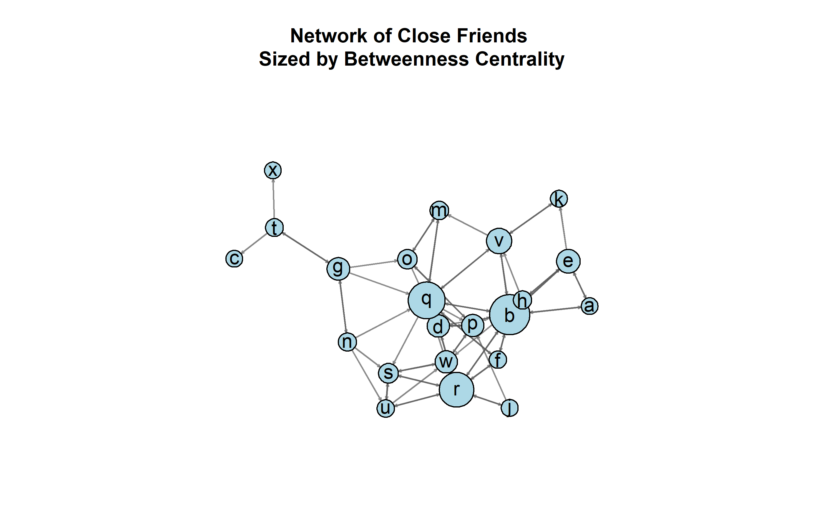
Figure 13.1: A directed network of self-reported friendships between students, sized according to betweenness.

Consider the visualization of the directed network in 13.1. The friends network consists of ties structured from one of three questions that students answered to denote close friends in class. Given the network’s structure and the betweenness centrality of each node, it seems apparent that three nodes dominate the network: q, r, and b. But is that level of centralization special to this class’ network, or is this something that we would normally expect for a network this size? Is it something that we would normally expect for a network with this size and number of edges? Is it something that we would normally expect for a network with this size and distribution of dyads? We could state, therefore, the null hypothesis for each as the following:

H₀: There is no difference between the measure of betweenness centralization in the friendship network and the betweenness centralization measures in networks of this size.

H₀: There is no difference between the measure of betweenness centralization in the friendship network and the betweenness centralization measures in networks of this size and number of edges.

H₀: There is no difference between the measure of betweenness centralization in the friendship network and the betweenness centralization measures in networks of this size and distribution of dyads.

We can compare each CUG test run on betweenness centralization with a null distribution conditioned on size, edges, and dyad census.

# Condition by size
cug.test(dat = friend, 
         FUN = centralization,
         FUN.arg = list(FUN = betweenness), 
         cmode = "size")
# Condition by edges
cug.test(dat = friend,
         FUN = centralization,
         FUN.arg = list(FUN = betweenness), 
         cmode = "edges")
# Condition by dyad census
cug.test(dat = friend,
         FUN = centralization,
         FUN.arg = list(FUN = betweenness), 
         cmode = "dyad.census")

We present an example of the raw CUG test output conditioned on size below followed by organized results for all three conditions (see 13.4). Output for a CUG test includes information on the parameters included in the test. In the example below, the first four lines of the output indicate that network size served as the condition upon which to simulate networks; the network data were directed (digraph); the diagonal was not used (meaning that no loops were considered in calculations or simulations); and, the test generated 1,000 simulated networks (the default for this function). The lower portion of the output gives the observed value of betweenness centralization (\(C_B\)=0.17) for the network being tested. The next two lines list the proportion of simulated networks with measures that are greater than or equal to the observed value, and the proportion with measures that are less than or equal to the observed measure, respectively. In this case, all the measures in the null distribution of simulated networks were less than or equal to the observed value of betweenness centralization. Normally, we can examine the proportions in much the same manner as a p-value in a standard statistical test. For reporting purposes, p-values cannot theoretically be equal to zero. For that reason, it is a good practice to report zero values of p as some arbitrarily small value such as p<0.0001. The following table presents the results for all three tests.

Univariate Conditional Uniform Graph Test

Conditioning Method: size 
Graph Type: digraph 
Diagonal Used: FALSE 
Replications: 1000 

Observed Value: 0.1700113 
Pr(X>=Obs): 0 
Pr(X<=Obs): 1 

Table 13.4: Output from CUG Tests Conditioning on Size, Edges, and Dyads

Betweenness	Percent Greater	Percent Less
0.17	0.000	1.000
0.17	0.268	0.732
0.17	0.458	0.542

If you so desire, it is possible to produce a graphical representation of the comparison that is being implemented to run the test. This step is an optional one and it will not contribute greatly to the analysis. However, some may find it helpful to be able to see the comparison between the measure taken on the network, and the distribution of measures taken on the various simulations. Generating the graphical representation is a matter of plotting the test. The script below produces three plots, side-by-side. This step is done by using the par(mfrow = c(1, 3)) to set the plot area to have one row and three columns. Each plot consists of the test name and an optional title (main).

par(mfrow = c(1, 3))
plot(cugBetSize, 
     main = "Betweenness \nConditioned on Size")
plot(cugBetEdges, 
     main = "Betweenness \nConditioned on Edges")
plot(cugBetDyad, 
     main = "Betweenness \nConditioned on Dyads")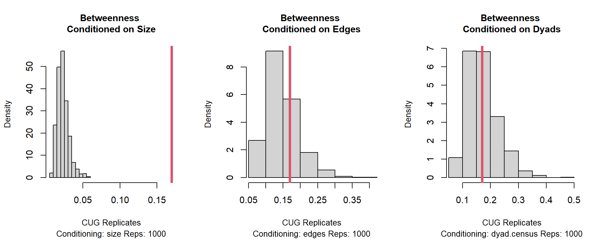

Figure 13.2: CUG Plots Conditioning on Size, Edges, and Dyads

The resulting histograms, pictured in 13.2, provide an intuitive representation of how the observed measure of betweenness centralization compares with the distributions of measures of the simulated networks. The vertical red line represents the observed measure and its relationship to the null distributions. In this case, the difference between the original network’s betweenness centralization is substantially greater than are those taken of the simulated networks of the same size. The histograms, however, demonstrate no statistically significant differences for networks conditioned on the same size and the same number of edges (density) as the friend network, or networks of the same size and the same number of dyads as the friend network. The latter two histograms illustrate that we cannot rule out the null hypothesis that the friendship network is the same as what we would expect from networks of the same size and density, or networks that are the same size and and have the same number of dyads. We can rule out the null hypothesis that betweenness centralization for the friend network is what we would expect for networks of the same size. This result is likely due to the way density and the number of dyads are not restricted when the networks are conditioned on size alone and were likely very different from the others.

13.3.2 Bivariate Tests Using CUG

Analysts can use conditional uniform graph tests with multiple networks for bivariate and multivariate statistical tests as well. A fundamental bivariate test that researchers use frequently is the correlation test. Correlations provide a measure of relationships between variables and can be used to summarize the amount of similarity between pairs of networks. Although correlation is a descriptive measure in statistics, there is an associated test. Before running a correlation test, the correlation value is normally symbolized with the letter “r” or, when referring to populations, the Greek letter Rho (\(\rho\)). Here, we use “r” to describe correlations between networks. In either case, correlation reflects the strength and direction of a relationship between two variables. In network analysis, those variables are embodied by networks.

Correlation Cheatsheet

• Correlation is generally expressed as a two digit decimal.
• Correlations may take any value between negative one (-1) and one (1).
  • -1 and 1 both indicate a perfect relationship (or redundant information!).
  • 0 indicates no relationship.
• The absolute value of the correlation indicates the strength of the relationship.
• The sign of the correlation (- / +) value indicates the direction of the relationship.

It is also helpful to think of correlations in terms of how strong or weak they are. This way of thinking provides a more intuitive means of expressing what the correlation value indicates about the relationship between variables. 13.5, below, provides some rules of thumb for interpreting and reporting correlation values.

Table 13.5: Rule of Thumb for Reading Correlation (Absolute) Values

Correlation Value	General Interpretation
|r| = 1.0	Perfect Correlation
0.80 < |r| < 1.0	Very Strong
0.60 < |r| < 0.80	Strong
0.40 < |r| < 0.60	Moderate
0.20 < |r| < 0.40	Weak
0.00 < |r| < 0.20	Very Weak
|r| = 0.00	No Correlation

The correlation test was designed to assess whether the correlation value is meaningful in the data that are being used. If the test indicates that the correlation value is not “meaningful,” then what we have learned is that we cannot rule out the possibility that the finding is spurious and no relationship actually exists. By running a correlation test, we are essentially double-checking to see whether a particular correlation is worth reporting. If the p-value for the correlation test is statistically insignificant (by convention, less than 0.05), then we treat the correlation as indeterminate. (We do not, however, report the value as zero.)

Testing correlation between networks in R is fairly straightforward and similar to the tests covered above using centralization. Although the correlation test will provide correlation values, it is a good idea to produce them separately.

Before going too far into how to calculate and test a correlation, it is important to highlight an important caveat. Each of the networks should be composed of the same nodes (people, organizations, etc.), and they should be in the same order if they are to be legitimately compared. Correlations between networks consisting of entirely different entities are not meaningful, since we are seeking to compare how similar or different the pattern of ties are for each node in one network with the same nodes in another. In other words, analysts only should calculate correlations between networks that represent differing sets of relationships for the same set of nodes. When statnet compares networks, it compares nodes based on the order in which they appear. The correlation function does not pay attention to vertex names and will not check to make sure that the networks consist of the same set of nodes and in the same order. So, while it is possible to get statnet to run a correlation on two networks of the same size but comprised of entirely different entities (e.g., people and organizations), the resulting correlation would be meaningless.

The defaults for the statnet’s correlation function, gcor(), are listed below.

gcor(dat, dat2 = NULL, g1 = NULL, g2 = NULL, diag = FALSE, mode = "digraph")

At its simplest, the gcor() function requires only a list of two or more networks that are comprised of the same node set. The function will produce correlation matrices when used with multiple networks, or a correlation value when using only two networks. As is standard for statnet, the gcor() function defaults to reading the networks as though they are directed (mode).

gcor(dat = know, dat2 = buddy)

[1] 0.5155708

The g1 and g2 arguments are used to identify which elements (e.g., networks) of a list to use when calculating a correlation value. In the first example below, the correlation between the (directed) “know” and “buddy” networks is measured. In the second example, two of the three networks (“know” and “buddy”) are again selected, this time from a list of networks. The third example produces a correlation matrix.

nets <- list(know, buddy, friend)
gcor(dat = nets, g1 = 1, g2 = 2)

[1] 0.5155708

To make the output more legible, the third example is nested within the round() function to reduce the output to two digits. 13.6 provides a cleaner version of the correlation matrix of the three relationships.

round(gcor(nets), digits = 2)

     1    2    3
1 1.00 0.52 0.25
2 0.52 1.00 0.51
3 0.25 0.51 1.00

Table 13.6: Correlation Matrix for Aquaintances, Buddies, and Friends

	Buddies	Close Friends
Know Name	0.52	0.25
Buddies	1	0.51

Correlation coefficients help empirically describe relationships. They do not provide, however, an indication of whether an observed measure of a relationship is just what we would expect from a pair of “similar” networks. Testing the correlation value provides an indication of whether that measure essentially is what we would expect in networks “of that sort.” The first decision, then, is in deciding what “networks of that sort” means.

Traditional (parametric) correlation tests are designed to take the amount of variation in the sample into account in order to estimate whether the sample’s observed correlation value is likely to exist in the wider population the sample represents. The null hypothesis is then stated as either “no relationship,” or “the correlation value between the two variables does not exist in the population.” Using “r” as the symbol for correlation, this is more succinctly stated as “r=0.”

For conditional uniform graph tests, we generally mean networks of the same size and maybe some other description. As with CUG tests, the correlation value for the original network pair is compared with the correlation values for all pairs of simulated networks. What we actually test is whether the strength and direction of the relationship (the correlation) that we observe between two networks is generalizable to similar networks. If we fail to reject the null hypothesis, we are saying that we cannot rule out the possibility that there is no difference between the measure we calculated and what we would expect from any two randomly selected networks of a certain type. The following are three alternatives for stating the null hypothesis (\(H_0\)) for this test. If we fail to reject it, we are saying that we cannot rule out that the correlation value we observe is spurious.

H₀: r=0

H₀: There is no relationship. (The observed measure is spurious.)

H₀: The correlation value of the network is the same as the correlation values between randomly simulated networks of similar __________.

R users should note a few differences between the two functions.³ One of the major differences between the two functions is the modes used for conditioning the simulated networks. Though similar, the options are not necessarily the same for both functions. The older function’s options allow analysts to condition networks based on size alone (order), size and tie probability (density), or size and bootstrapped degree distributions (ties). The default for this function is to condition networks on density. Therefore, if cmode (i.e., condition mode) is not specified, or if a user enters something the function does not recognize (i.e., anything that is not order, density, or ties), cugtest() will condition on density.

Table 13.7: Differences in Conditioning between cug.test and cugtest

Meaning	cug.test (newer)	cugtest (older)
Number of nodes in the network	“size” (default)	“order”
Distribution of edge values in the network		“ties”
Distribution of edge values, or number of edges in the network	“edges”
Density of the network		“density” (default)
Number (or value) of dyads the network	“dyad.census”

Another difference between the two is that this older version allows analysts to specify which networks in a list to test. Unlike the gcor() function, which can produce a correlation matrix from a list of multiple networks, statnet does not currently produce a matrix with the results of correlation tests using conditional uniform graphs. Users have to estimate each test individually, as in the example below, or employ in a function to produce such a table. By default, statnet will select the first and second networks in the list (g1 = 1 and g2 = 2). Users have to specify any other combination of networks.

In the example below, correlation tests are run on a list of three networks (know, buddy, and friend). The know network is first, buddy is second, and friend is third. The function will see them, therefore, as networks 1, 2, and 3. The name of each object is, of course, up to the individual running the analysis. In this case, we named each test object in a way that helps keep track of which comparison is being run in each test and the conditions upon which the simulations are produced. This approach can be helpful since the output is savable and the network names and type of conditioning are not available in the output.

nets <- list(know, buddy, friend)

corOrd13 <- cugtest(nets, gcor,
                    g1 = 1, g2 = 3,     # The first and third network
                    cmode = "order")
corOrd12 <- cugtest(nets, gcor, 
                    g1 = 1, g2 = 2,     # The first and second network
                    cmode = "order")
corOrd23 <- cugtest(nets, gcor, 
                    g1 = 2, g2 = 3,     # The second and third network 
                    cmode = "order")

For demonstration purposes, the next output depicts the results of only the first of the three tests. Unlike the newer cug.test() function, cugtest() does not provide information about the mode used for conditioning, whether the network was read as directed or undirected, or whether the diagonal (indicating the presence of loops) was included in the test. What this output provides, however, is still sufficient for performing the test and interpreting the results. Specifically, the output includes the p-values that were calculated in the same manner as the newer version, the number of simulations that were generated (Replications), the correlation value (Test Value), and a summary of the correlation values calculated for the simulated networks.

The p-values reflect what can be seen when comparing the correlation value for the “know” and “friend” networks with those of the simulated networks. At no point is the correlation between simulated networks greater than 0.25. It is, rather, uniformly much lower. From this, we may conclude that it is safe to reject the null and conclude that the observed correlation between “know” and “friend” is not spurious when considered in comparison to networks of this size.

corOrd13   <- cugtest(nets, gcor, g1 = 1, g2 = 3, cmode = "order")
summary(corOrd13)

CUG Test Results

Estimated p-values:
    p(f(rnd) >= f(d)): 0 
    p(f(rnd) <= f(d)): 1 

Test Diagnostics:
    Test Value (f(d)): 0.2493995 
    Replications: 1000 
    Distribution Summary:
        Min:     -0.1864245 
        1stQ:    -0.0338401 
        Med:     0.0003852113 
        Mean:    -0.001926882 
        3rdQ:    0.0279094 
        Max:     0.1199181 

It is also possible to plot the distribution of simulation values using plot(corOrd13), though the plots will appear somewhat different from the newer versions. As with other CUG tests, however, the plots are best only for illustration purposes and unnecessary for inference.

13.4 Quadratic Assignment Procedure (QAP)

Quadratic assignment procedure (QAP) is similar to CUG, in that it employs simulation in order to generate a distribution of hypothetical networks. However, whereas CUG controls for a network condition such as size or density, QAP controls for network structure (Mantel 1967; Hubert and Schultz 1976; Krackhardt 1987b, 1988). QAP is useful for running a variety of statistical functions and, until recently, has been one of the most popular (and, therefore, widely accepted) methods for assessing statistical significance with network data. Below, are three of the options available in statnet.

QAP is similar to bootstrapping in that it builds its own distribution using network simulations that are based on the network being estimated. This particular simulation process is referred to as a permutation test, and it is designed to mimic all of the scenarios that would be possible if everyone were able to switch places in the social order. In other words, the rows and columns in the network matrix are shuffled (i.e., permuted) randomly while names (and all their corresponding attributes) remain in the original order. This process essentially changes the node with which a particular name and set of attributes is associated without disturbing the underlying structure (See Figure 13.3 for an example of a permuted network). This random rearrangement is repeated to create a large number (usually hundreds or thousands) of simulated networks, which are then analyzed in the same manner as the original network in order to create a distribution of statistical measures that can then be compared to the measures calculated for the observed (i.e., actual) network. As with CUG tests, the proportion of measures in the distribution that are greater than, and less than the measure taken from the original network are then produced to give “p-value”-type information. If the observed measure occurs sufficiently infrequently (p < 0.05) within the distribution of simulated networks, then we can reject the null and conclude that the observed statistics are not likely to have occurred by chance alone.

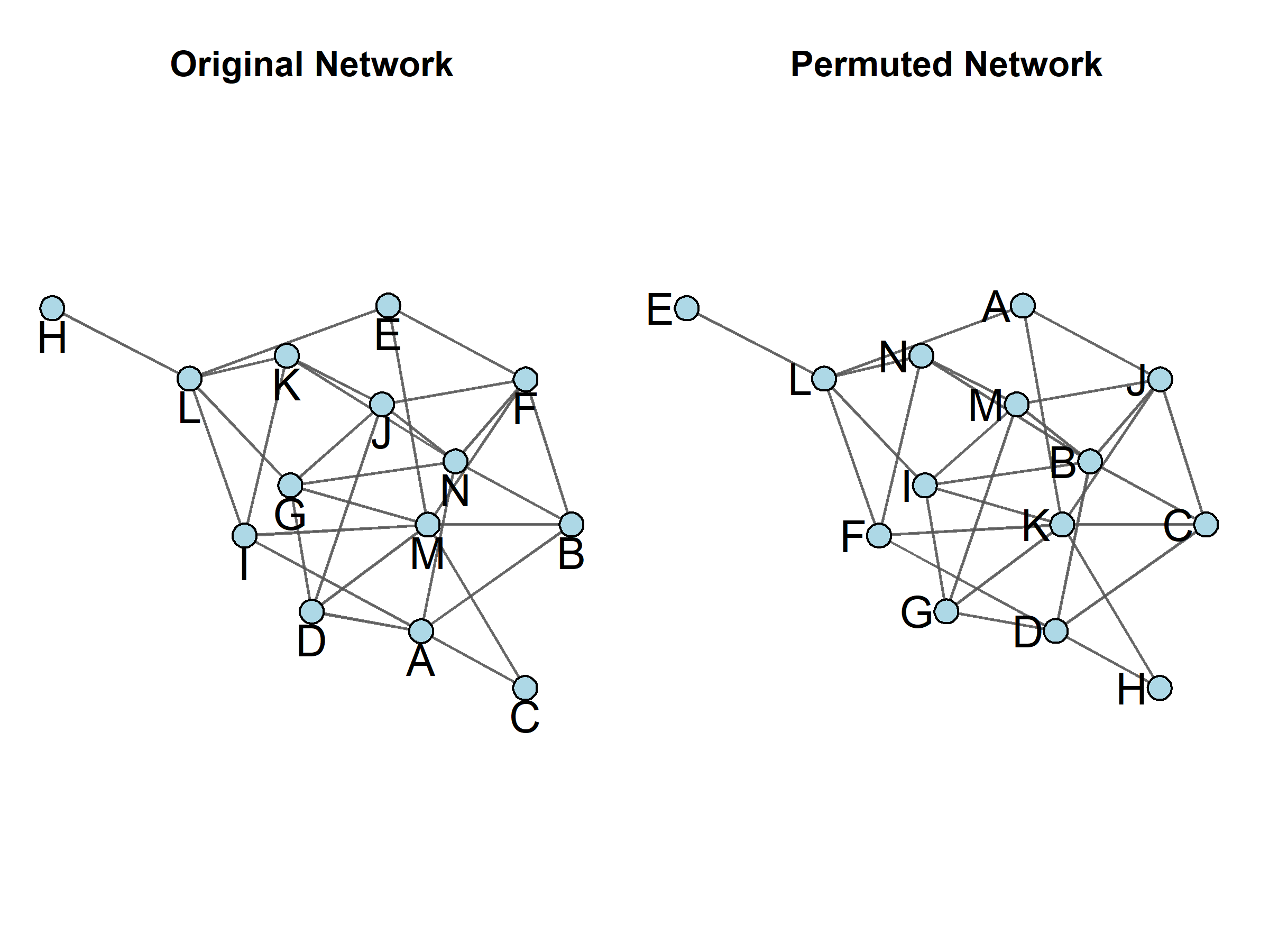
Figure 13.3: Two Permutations of the Same Network

The essential difference, then, between CUG and QAP is that CUG controls for networks of a “similar type,” whereas QAP controls for the particular pattern of interrelatedness (i.e., network structure) in the original networks. When using QAP, we are ultimately asking whether the result of the test we are running is spurious, given the autocorrelation that is normally inherent in networks. The procedure accomplishes this by observing the interdependencies that are apparent through the network structure, and then essentially reshuffling the nodes along with all their attendant attributes among the various positions within that structure. The idea behind this is that the network’s various interdependencies remain in place, but the permuted networks are used to see whether the values we calculate would still be the same if the entities themselves were not interdependent in the same ways.

For an analogy, imagine that everyone in a network was moved to some new spot in the social order in the network. If the ties within the network are fairly dense, with a lot of symmetry, it is much less likely that permutations of the network will result in large differences in the social order. This implies that the resulting correlations would not reflect a great deal of difference either. To illustrate, consider an extreme case. A friendship network that forms a clique would not change at all if all the positions were swapped around, since everyone in the clique is already adjacent to everyone else. So, permuting the network likely would not produce any differences in terms of relative positions in the structure of the network.

13.4.1 Bivariate Tests Using QAP: Correlation

Correlation values are calculated the same way, regardless of whether one is using CUG or QAP. It is the test and its accompanying assumptions that differ. When calculating the level of correlation between two networks, the first step is to compute the correlation coefficient between corresponding cells. Next, one of the networks is randomly permuted and the correlation is recalculated. This step is carried out hundreds or thousands of times in order to compute the proportion of times that a random measure is larger than or equal to the observed measure calculated in the first step. A low proportion suggests that a correlation between networks is unlikely to have occurred by chance and the correlation value is thus not spurious.

Consider, for example, the organizational convergence networks, which describe the connections formed within and between two organizations that are in the process of merging into one. Table 13.8, below, presents the three types of relationships identified as being important to the daily functioning of the institution. One concern that arises when conducting a survey of this sort is whether respondents are reading closely when answering each question and providing information appropriate to each question or just giving the same set of alters each time.

Table 13.8: Organizational convergence network

Network Name	Survey Question
commun	“With whom do you communicate to perform your work?”
collab	“With whom do you collaborate?”
esteem	“With whom would you like to work in the future?”

Again, we’ve stored these as .rda files, which we can read using the load() function.

load("Communication.rda") # Loads as "commun"
load("Collaboration.rda") # Loads as "collab"
load("Esteem.rda") # Loads as "esteem"

Because it measures relationships, one can think of correlation as providing a description of how much overlap exists between each of the networks. We may use correlation, therefore, to check whether respondents provided largely the same answers for each of the three questions. We would expect some overlap (i.e., maybe a weak to moderate correlation) if respondents answer each of the questions with a different type of relationship in mind. But, strong, very weak, or negative correlations would be a sign that we did a poor job of eliciting the various relationships. Table 13.9 presents the results of the correlation measures among the three networks.

[1] 0.6009021

          1         2         3
1 1.0000000 0.6009021 0.4092608
2 0.6009021 1.0000000 0.3891069
3 0.4092608 0.3891069 1.0000000

Table 13.9: Table: Correlation Matrix

	Collaboration	Esteem
Communication	0.6	0.41
Collaboration	1	0.39

The correlation matrix in Table 13.9 demonstrates that the relationship between communication and collaboration is moderate to strong. This result makes sense, as we would expect that those who collaborate also communicate. But, not all who communicate useful information are also collaborating in their work. Collaboration and communication are also manifest ties, meaning that they are ties that exist in some tangible sense. The “esteem” network is more theoretical, and this becomes clear when one considers that the relationships between the manifest, and more tangible, networks correlate only weakly with the more nebulous idea of who people would like to work with in the future.

The question that may arise at this point is just how much we should trust these correlation values. The test associated with Pearson’s correlation assesses whether the correlation value is “real,” or meaningful. The qaptest() function operates in a manner that is very similar to that of cugtest(). In its current form, the qaptest() function can simulate only the interaction between one network pair at a time. It is, therefore, necessary to specify which networks are being compared each time. The example below gives examples of how we would test correlation values for each of the network pairs.

nets <- list(commun, collab, esteem)

cortest12 <- qaptest(nets, gcor, g1 = 1, g2 = 2)
cortest13 <- qaptest(nets, gcor, g1 = 1, g2 = 3)
cortest23 <- qaptest(nets, gcor, g1 = 2, g2 = 3)

The format of the qaptest() function’s output is similar to the cugtest() results. The label QAP Test Results indicates the test results, with p-value approximations, the correlation value for the networks being compared, the number of simulated networks that were produced, and the distribution of correlation values between simulated networks. One can read and interpret the output, therefore, in the same manner as with CUG tests. As with other tests, users also can produce the distribution plot for the QAP correlation test.

summary(cortest12)

QAP Test Results

Estimated p-values:
    p(f(perm) >= f(d)): 0 
    p(f(perm) <= f(d)): 1 

Test Diagnostics:
    Test Value (f(d)): 0.6009021 
    Replications: 1000 
    Distribution Summary:
        Min:     -0.05672636 
        1stQ:    -0.0152203 
        Med:     -0.0006662233 
        Mean:    -0.0001104733 
        3rdQ:    0.01334881 
        Max:     0.06347951 

13.4.2 Multivariate Models using QAP

Testing the significance of univariate network descriptors, as with CUG, or testing bivariate descriptors, which is possible in both CUG and QAP, are powerful for their ability to validate or qualify the results of the measure or a test. Multivariate techniques, on the other hand, provide the option of using multiple variables to predict or explain an outcome. The use of multiple variables offers a powerful advantage over univariate or bivariate techniques, as the multiple predictors hold the potential to explain a great deal more about some outcome of interest.

Multivariate techniques offer the advantage of accounting for a great deal more of the complexity that is inherent in social relations. The techniques presented below, and in the following chapters, are means of conducting multivariate analyses with network data. The two techniques presented below are more classical approaches to the problem of conducting multivariate network tests. Although both CUG and QAP may be used to create the null distribution for either approach, we present only the more commonly used used QAP approach.

Below are two forms of multivariate regression: logistic regression and ordinary least squares (OLS) regression. The major difference between the two is in how ties in the network functioning as the dependent variable (i.e., the network being predicted or explained) are measured. The type of regression you choose, therefore, should reflect the way ties are measured in the dependent network. For example, in a scenario for testing whether family ties, prior communications, or business ties predict (or explain) operational collaborations between group members, the outcome of interest is operational collaborations.

Logistic regression is designed for binary data and is suited for predicting or explaining the odds that a tie will form between any two nodes, given other factors. One should use it when the outcome network has tie values of only one or zero. In terms of the example presented in the QAP correlation section, “collaboration” only would be measured as one (a collaboration is observed) or zero (there was no collaboration observed). Multiple OLS regression, on the other hand, is best suited for explaining or predicting continuous measures. It is therefore better suited for use with dependent networks with tie values that could take any number. In the operational collaboration example, multiple linear regression would be appropriate if one measures the degree of collaboration (e.g., number of observed collaborations, “strength” of the collaboration, layers of collaboration) rather than just the simple presence or absence of collaboration ties.

Note that the ties within the predictor networks (those networks being used to predict or explain the outcome network) may be either binary or continuous for either method. Numerous options and interpretation caveats go with either regression method. The descriptions below are provided only as a very general introduction. To use either of these tools well, it is advised that users consult any standard statistical text for properly applying either type of regression. Aside from the fact that here we use networks rather than independent observations, the rules for applying these techniques are fairly similar.

Multiple regression - both OLS and logistic - allows analysts to use multiple predictor variables to predict or explain what we should expect from some other variable of interest. That is to say, we can use more than just one variable when trying to understand another. This is important when one considers that, in reality, outcomes tend to be much more complex than what a single predictor can capture - no matter how critical or important that predictor may be. Multiple regression makes it possible to account for the relationship between the predictors and the outcome while also controlling for the interrelationships between the predictors themselves. If you estimate three regression models, each with a different predictor, and then a fourth with all three predictors together you will notice a difference between what each of the predictors say about the outcome individually, and what they say when they are all included in the same model. This is because each of the predictors may be themselves related to one another.

If predictors are even somewhat related, then the information they contribute about the outcome variable will likely overlap to some degree. When taken together, the redundancies are taken into account and each variable’s unique contribution is much more precise.

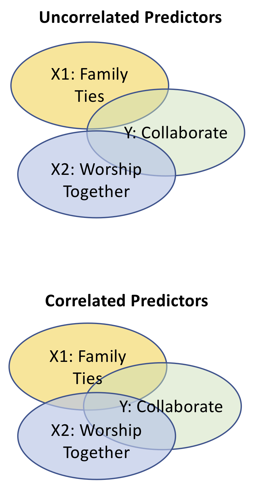
Figure 13.4: Uncorrelated and Correlated Predictors in a Regression

More advanced tools are presented in subsequent chapters. They are considerably more involved and each is designed with specific analytic goals in mind. The following examples offer a good place to start for those who are just beginning to explore the potential of multivariate analysis. Once you have established a comfort zone around the following tools, you will likely have a much easier time in grasping the nature of ERGMs, SAOMs, latent space models, multilevel models, and other advanced techniques that are now available to network analysts.

13.4.2.1 Multiple OLS Regression - Basics

Multiple ordinary least squares (OLS) regression is a powerful technique for estimating a continuous outcome. We generally think of the estimates that a regression produces as either predicting or explaining that outcome. The name, “ordinary least squares,” refers to the way the prediction fits the patterns evident in the data. For a model to be a “good fit,” it should, overall, have the least (smallest) squared differences between what the model predicts and what the data show. There are other methods for fitting a regression model, but this is probably the most common and best understood.

Fundamentally, multiple regression uses the information contained in a set of independent variables (i.e., predictors) to make some prediction about a dependent variable (i.e., outcome). In theory, the variation in the outcome depends on the behavior of a set of predictors that are relatively independent of one another. Analyst use this tool to predict or explain what we should expect to see in some outcome if there is a change in one or more of the predictors.

The generic equation for a regression model is:

\[ Y_i= \beta_{0} + \beta_{1} X_{1} + \beta_{2} X_{2} + \beta_{3} X_{3} + ... + \beta_{k} X_{k} + \varepsilon \]

In a regression model, \(Y_i\) represents the outcome, or dependent variable, that is being predicted or explained. The explanations are given by the \(\beta_{i} X_{i}\) chunks of the model. The \(X_{i}\)s represent the predictors and the \(\beta_{i}\)s represent the slope, which tells us how much and in what way we should expect the outcome to change for each one unit change in the particular predictor with which it is associated. When we specify (i.e., construct) a regression model, we only select the outcome and predictors (\(Y = X_1 + X_2\) or \(earnings = experience + age\)). The betas (\(\beta\)) are calculated by estimating the regression. For example, if the beta for the predictor “experience” (in years) is calculated to be 250 (\(\beta_{experience} = 250\)), then we would expect that, for each additional year of experience, the outcome (in this case, earnings) would increase by 250, holding the other predictors constant.

That last bit (holding the other predictors constant) is important. It means that we are using the model as a relatively full description of what may predict or explain changes in an outcome. But, if we use just one of the variables to describe the expected changes in the outcome, then we should also acknowledge that this is what we would expect in the presence of the other variables. In other words, this is just one part of the story of what makes that outcome change.

There are a few other elements to the equation that should be noted. The ellipse, followed by “\(+ \beta_{k} X_{k}\)” is included to point out that it is possible to add any number of predictors to a model, within certain limits. There are a number of important considerations to selecting a reasonable and valid number of predictors for a regression model, and readers are strongly encouraged to seek that information in a text that deals more specifically with regression techniques and considerations.

The (\(\beta_0\)) symbol is referred to in the output from estimating a regression as the “intercept.” It may be interpreted as the value of the outcome when the values of all of the predictors are zero. An error term (\(\varepsilon\)) is also included in the formal regression model. The error is not something that analysts will calculate. It is merely included to make the equation balance and acknowledge that we are only explaining a portion of what makes the outcome vary. There will always be something that we miss in our description (and, thus, in our models).

13.4.2.2 Multiple OLS Regression using QAP

Some important differences exist between estimating a multiple regression with standard, randomly selected data and estimating one with network data. One of these considerations involves the number and type of simulations that are used for assessing the model. The example below focuses on introducing quadratic assignment procedure (QAP) for multivariate models. The QAP procedure that was initially introduced by Krackhardt assumes that all of the predictors are independent of one another (uncorrelated). The problem with that assumption is that relationships between predictors are common in multiple regression, but they reduce the accuracy of the original QAP test.

Because the assumption of independent predictors is unrealistic in most circumstances, a newer QAP approach called “double semi-partialling” (Dekker, Krackhardt, and Snijders 2007) was developed to provide a more robust permutation test that better accounts for the correlations between predictors. This was done through a modification of QAP that permutes the regression residuals (the difference between what the model predicts and what the data actually show in each observation) for each of the predictor variables over the network structure. This creates a permutation method that is more effective in reducing Type I error rates than other available QAP approaches.

We cannot emphasize enough that this overview of multiple regression and QAP multiple regression is very superficial. Please look into some of the suggested readings at the end of this chapter if you are not already familiar with either method. They can be very powerful analytic techniques, but the analysis also may be very nuanced in its execution if one hopes to produce an accurate interpretation of the output.

13.4.2.3 Options and Defaults in QAP OLS Regression

The help section for netlm() offers the following defaults for the function:

netlm(y, x, intercept = TRUE, mode = "digraph", diag = FALSE,
    nullhyp = c("qap", "qapspp", "qapy", "qapx", "qapallx", "cugtie", "cugden",
                "cuguman", "classical"), 
    test.statistic = c("t-value", "beta"), 
    tol = 1e-7, reps = 1000)  

The netlm() function requires, at minimum, a dependent variable (y) and at least one predictor (x). The dependent variable must be entered as a matrix of valued ties. This point is important to the analysis, as you will need a continuous dependent variable to run an OLS regression. If a network object, rather than a matrix, is entered as the dependent variable (y), then the tie values will be ignored and the network will be considered to be composed of binary ties. Users will receive no warning about this, and as previously discussed, multiple OLS is designed to predict tie values; thus, a dependent network composed only of 0s and 1s could result in misleading results.

By default, the netlm() function reads the input networks as directed and not containing loops (i.e., diagonal values). If you are working with undirected data or data with loops, you will need to modify the mode or diag parameters to reflect those network features. The function will not automatically adjust how it reads in data.

With the exceptions of y, x, mode, and diag, it is generally a good idea to leave the default arguments as they are when running a regression. That said, statnet allows users to modify a number of additional parameters that may be helpful under some very specific conditions. Users may change the type or manner in which the networks that are used for hypothesis testing are simulated, the speed and specificity of the test, and some control of the model’s ability to converge on “accurate enough” estimates. Users should consider changes to these parameters carefully before making them, as they will usually change major assumptions under which the model is estimated.

As with other functions in statnet, the number of permutations defaults to 1000 (reps = 1000). Changes in this parameter will not affect the accuracy of the estimates in the regression output, but it will affect your ability to assess their significance. A larger number will generally make it easier to differentiate between whether the null should or should not be rejected. The tradeoff, especially with larger networks and multiple regression models, is that the regression can take a while to run. In the initial model-fitting phase, where a user may wish to see if they can get a model to run, it is fine to lower the number of permuted replications for the sake of speed. However, in the interest of avoiding a false positive (Type I error), any final models should be run with a larger number of iterations (>1,000).

Other defaults include the option of whether to use the intercept, the type of generated networks to use as comparison for testing the null hypothesis, as well as some more nuanced refinements to the network simulations. By default, netlm() includes an intercept in the regression. This is standard for a regression and its removal only should be done under a very limited set of circumstances, as doing so would be unrealistic in most situations.

The nullhyp options include a variety of QAP and CUG simulations that will be used to simulate networks to be used to test the null. At the time of this writing, qap (the default) and qapspp function identically and use the double semi-partialling approach discussed earlier. However, the netlm() function also allows users to apply selectively some less-used variations of QAP. In many cases, the other options will have a higher Type I error rate than the double semi-partialling approach. Under some - very limited - conditions, users may wish to independently permute each of the predictors (qapallx), or permute one predictor at a time while holding the others constant (qapx). On most occasions, QAP permutes the predictor variables. If there is a good reason for doing so, users may alternatively elect to permute the outcome (qapy). Under other special conditions, users also are offered a variety of conditional uniform graph simulation methods, such as simulating networks of the same order (cug), density (cugden), or tie distribution (cugtie). There is even an option to run a regression without simulating networks to test the null (classical). However, we do not recommended this under any circumstances since the fact that you are using network data violates the assumptions behind the least squares modeling being used to assess significance, which substantially raises the probability of committing a Type I error.

The remaining parameters that may be set offer means of tweaking a regression either to have closer comparisons for hypothesis testing or to produce estimates under difficult circumstances. The test.statistic argument allows the user to select between using a "t.value" distribution and a "beta" distribution when generating simulated networks. The simulated networks that are generated to test the null hypothesis are drawn from a universe of possible networks, had some things been just a little different. This approach is somewhat like looking at models of alternate realities, each of which is based on the one that we have observed in the networks we are analyzing. Monte Carlo procedures are used to generate the simulated networks. Rather than subscribe to the “anything is possible” line of thinking (a uniform probability distribution), the simulated networks are based on the originals with most simulations bearing a fairly strong resemblance to the original. They are drawn from a realm of possibilities that has most of the networks’ possible morphologies being just a little different and progressively fewer being very different.

The way that the possible network morphologies or permutations are distributed should reflect the actual probabilities that the networks may take on such structures. The problem with this is that we almost never possess such knowledge. It is very difficult to know what could have been under unlimited hypothetical scenarios. That said, in some cases, we might have some idea that there should be even odds as to whether the network could have deviated in one direction or another. Alternatively, perhaps, we may have prior knowledge that chances are better that the networks would be different in a particular way than another. In such cases, we can design the comparisons to be either evenly distributed around the original network or in a manner that favors a particular morphology over another. That is the purpose behind the two test.statistic options.

The t-distribution should be adequate, under most circumstances, when selecting a distribution for the test statistic. The t distribution ("t.value") provides a symmetric probability distribution, meaning that any value drawn at random from the distribution is equally likely to be either above or below the distribution’s mean. The beta distribution (beta), on the other hand, is used when analysts have prior information that gives them reason to believe that certain states are more likely than are others. It can take a range of shapes, including symmetric, with the shape depending on the prior information gained through - in this case - parameters of the network being analyzed. When it takes on a skewed shape, it assigns a greater probability for values falling in one direction rather than the other - greater or less than the median. In either case, the simulated networks affect only the networks that are generated for hypothesis testing purposes.

An argument that may affect the regression estimates of the intercept and beta values is “tolerance.” By default, tolerance is set very close to zero. The tolerance is small because it is used as a parameter that guides the algorithm in assessing whether calculations have begun to improve so little in each iteration that we may judge then to have converged upon the answer. In essence, the tolerance is a standard used as a stopping point for the algorithm. The clear tradeoff is that smaller tolerance values may take longer to converge, but greater values may - sometimes substantially - decrease accuracy.

The netlm() function tolerance defaults to tol = 1e-7. We do not recommend users to modify this parameter; it should be adequate under most circumstances. If a model fails to converge, we strongly recommended that users first reevaluate the model, as that is frequently the source of the problem. Possible reasons for failure to converge include multicollinearity or an outcome with too little variation. But, if there is some reason why the model must remain as-is, then the tolerance may be adjusted upward by small increments. However, the upper tolerance limit for the tolerance should be somewhere around 1e-5 or 1e-4 and the output should be regarded with some skepticism at that point.

13.4.2.4 Estimating a QAP OLS Multiple Regression in R

For an example of multiple OLS regression, consider the class friendship and interaction networks introduced at the beginning of the chapter. Neither of these networks has valued ties, but we can create a network with tie values by adding network ties together. In this case, we will add three types of ties that express how much of an affinity people have for one another: people they know (know); people they like (buddy); and people they feel close with (friend). When added together, we have a “friendship” scale that ranges from not friendly (0) to very close (3). This step is accomplished as follows:

# Make a matrix to use as a dependent variable
friendship <- as.matrix(know) + as.matrix(buddy) + as.matrix(friend)

We can now estimate a QAP multiple regression since we have a network with valued ties (friendship) to use as an outcome. For our independent networks, we will use three: one that captures students who worked together in groups (groupWork), one that indicates students who had classes together (haveClass), and one that indicates students who tended to talk with and work with one another (WorkWith). Each of the predictor variables are binary, meaning that all tie values in the networks are either 1 (a tie is present), or 0 (no tie exists).

The resulting model may be written as:

\[Y_{friendship}= \alpha + \beta_{groupWork} X_{groupWork} + \beta_{haveClass} X_{haveClass} + \beta_{WorkWith} X_{WorkWith}\]

When using the netlm() function’s defaults, running the model is fairly straightforward.

set.seed(8675309)

nols <- netlm(friendship, list(groupWork, haveClass, WorkWith))

print(nols)

OLS Network Model

Coefficients:
            Estimate   Pr(<=b) Pr(>=b) Pr(>=|b|)
(intercept) 0.09013486 0.799   0.201   0.262    
x1          0.54500391 1.000   0.000   0.000    
x2          0.49071928 1.000   0.000   0.000    
x3          1.01990958 1.000   0.000   0.000    

Residual standard error: 0.6979 on 458 degrees of freedom
F-statistic: 190.2 on 3 and 458 degrees of freedom, p-value:     0 
Multiple R-squared: 0.5547  Adjusted R-squared: 0.5518 

We can call the output for a QAP multiple regression using either the print() or summary() commands. The print() command, which we use in our example, generates only the standard regression output, while the summary() command provides additional diagnostic measures, as well as which type of simulated network was used to create the null hypothesis distribution and the number of simulated networks in the distribution.

The regression output from netlm() does not retain or include the names of the variables used. When running a number of regressions, this can quickly become a problem, since many of the regressions will look alike. It is, therefore, important to either retain the R script used to run the test, make a note of the order in which you entered the variables, or both.

The F-statistic essentially tells us whether the model is more informative than if we were to simply consider the average tie value from the outcome variable (\(\mu_{friendship} = 1.10\)). In this case, the F-statistic is significant (\(p\leq 0.05\)). Thus, we can reject the null hypothesis that there is no difference between the information gained thorough using the model instead of the average tie value and conclude that the model is informative. We may, therefore, move on to consider the estimates that the model produced.

In the output from the friendship model, under “Coefficients:” x1 represents the first variable in the model (groupWork), x2 represents the second (haveClass), and x3 the third (WorkWith). It is apparent from the two-tailed p-values (Pr(>=|b|)) that each of the three predictors is statistically significant (\(p\leq 0.05\)), telling us that all three variables predict (or, if you prefer, explain) the tie values in the outcome network. The intercept, on the other hand, is not statistically significant and therefore cannot be interpreted. We can, however, plug the estimates into the model at this point.

\[Y_{friendship}= 0.09 + 0.55 *X_{groupWork} + 0.49 * X_{haveClass} + 1.02 * X_{WorkWith}\]

The interpretation of the variables in this model generally is done variable by variable, while holding the others constant. For example, we can interpret the variable WorkWith as predicting, “the value of a friendship tie would increase by 1.02 if students work and talk together in class, holding the other two variables in the model constant.” In other words, if two students share a tie in the WorkWith network, then we would predict that the value of the tie that they share in the friendship network would be at least 1.02, regardless of whether they have ties in the haveClass or the groupWork networks. In addition, because all of the predictors in this network are measured in the same way (all three are binary networks), we can also see that that WorkWith ties appear to be more strongly associated with friendship tie values than the other two types of ties. If we measured the predictor networks on different scales, then we could not draw such a conclusion.

Finally, we may wish to note the R-squared value. R-squared is a rule of thumb, and may be regarded an approximate measure of the variation in the outcome that is accounted for by the model. This value gives us an idea of how good our model predicts the outcome we are analyzing. In this case, we could state that this model accounts for roughly 55% of the variation in the value friendship ties in this network. Again, keep in mind that this is just a rule-of-thumb indicator and should not be taken too seriously.

13.4.2.5 Logistic Regression Using QAP

Logistic regression was designed to predict or explain binary outcomes. It is, therefore, best used to analyze networks with binary ties (i.e., tie values take a value of “0” or “1”). Like multiple OLS regression, the purpose of logistic regression is to describe the relationship between some outcome and the predictor variables that may relate to it. The major difference between the two is that logistic regression is designed for binary outcomes and, therefore, predicts the likelihood of a tie forming in the outcome network.

13.4.2.6 Options and Defaults in QAP Logistic Regression

The help section for netlm() offers the following defaults for the function:

netlogit(y, x, intercept = TRUE, mode = "digraph", diag = FALSE,
    nullhyp = c("qap", "qapspp", "qapy", "qapx", "qapallx", "cugtie", "cugden",
              "cuguman", "classical"), 
    test.statistic = c("z-value","beta"), 
    tol = 1e-7, reps = 1000)

As you can see, there is very little difference between the options in netlogit() and netlm() functions. The two differences are the y variable and the test.statistic. Because logistic regression is designed specifically for binary data, there is no problem with using a network object for the y variable. The netlogit() function will read network variables correctly, as being dichotomous. It remains important, however, to recheck the nature of the data being tested in order to account for directed networks and whether or not loops are present.

The other difference, the test statistics available used for modeling the simulated networks, is in the available distributions. The notable difference is the use of the z-distribution, rather than the t-distribution, as the default option. This is because z is better suited for use with dichotomous outcomes than the t-distribution. It is also a symmetric distribution and thus models values above and below the median as being equally likely. The beta-distribution is available in both netlm() and netlogit() since it we can use it to describe dichotomous or continuous data. As mentioned earlier, it allows for either symmetric or skewed distributions. Depending on prior information, as is present in the network data, the beta distribution may give more weight to values either above or below the median.

For most users, the test statistic options may not be necessary. Nevertheless, it is still important for those using the netlogit() function to review the options carefully and modify all that apply to the analysis being conducted and the networks being used to do so. For more information on each of the arguments within the netlogit() function, review the options and defaults section under the netlm() section of this text.

13.4.2.7 Estimating a QAP Logistic Regression in R

Estimating a logistic regression in R can be deceptively simple. If the observed network is directed and has no loops, then all that may be required is to list the networks being used as outcome and predictors. For an example, consider the organizational convergence network used in the QAP correlation example earlier in the chapter. Assuming that the organization would be interested in explaining why colleagues collaborate on projects, the other two networks could prove useful.

As it happens, the networks used in this example are undirected. In addition to the outcome variable (y) and predictor variables (x), it is important for the sake of accuracy to identify the networks as undirected (mode = "graph"). All other default settings are applicable to this analysis, so no further specification is necessary.

set.seed(8675309)

nlog <- netlogit(collab, list(commun, esteem), mode = "graph")

#Examine the results
print(nlog)

As with OLS QAP regression, the logistic QAP model for networks does not retain or include the names of variables. In the model above, recall that the outcome is collaboration, x1 is the network of communication ties, and x2 is the network of esteem ties. As with netlm(), either print() or summary() will call the regression output, with the latter calling additional diagnostic output.

The chi-square test of fit improvement provides a loose indication of model fit. A significant p-value for the chi-square test of fit improvement tends to indicate relatively good model fit. Although this is a good place to start in evaluating the model, there are other indications that also should be considered. In this case, the p-value is less than the conventional 0.05 threshold, indicating that there is some reason to believe that the model may be a good fit.

Each of the predictor variables, communication and esteem, are also statistically significant. The netlogit() output provides two forms of estimates. The coefficients listed under Estimate are the log odds of a tie in the output network, and the Exp(b) coefficients are the odds ratios, calculated by taking the exponential function of the log odds. For example, the exponential function of the estimate for community ties may be calculated by entering exp(2.920187). The odds ratios are provided for the user’s convenience. We can see that the estimates of the log odds for each of the variables is positive, indicating that the likelihood of a tie is more likely than not in each case. We can get an idea of just how much more likely when considering the odds ratios. For example, the odds ratio for communication is 18.5, indicating that - holding all other variables constant - a collaboration tie is 18.5 times more likely between offices that share communication ties than with those that do not. We can see that, as may be expected, communication ties appear to offer greater odds of creating a collaboration tie than do esteem ties in this network.

The pseudo R-square values offer a rough approximation of how well the predictors account for what we can observe in the outcome. We should note, however, that pseudo R-square measures are usually fairly conservative and, as with OLS regression, far from exact.

13.5 A Note on interpretation: Causality in Networks

Whenever employing statistical techniques to draw inference about the mechanisms that appear to drive the network in some fashion, it is best to be very careful when making statements about “causes,” regardless of whether or not the interaction, correlation, or other feature has been statistically verified.⁴ Generally, what analysts should keep in mind when working with social networks is that actual causes will be difficult, at best, to demonstrate (Doreian 2001). Nevertheless, if causes truly are what they are pursuing in their work, a few words of guidance may help.

Analysts can build solid analyses from a strong command of the context, culture, and actors under consideration. Background research is the worst topic on which to cut corners when analyzing networks. Preparation in terms of learning about the network will pay dividends when it comes time to interpret the results of any test or measure that one performs on a network. Similarly, preparation in terms of knowing theories that others have formed in their work with the same or somewhat similar networks will help to set up expectations and should alert analysts to situations that are surprising for their deviation from the norm. It is always helpful to know when something unexpected is taking place, and one generally will not recognize such things in the absence of background work. Background research functions primarily as a filter through which to interpret analyses.

In order to establish causal mechanisms, four essential factors must be in place (adapted from Shadish and Campbell (2002))

• A plausible argument
• Correlated predictor and outcome
• Temporal precedence
• Account for/rule out alternate explanations

The first item is relatively straightforward. It sets out that the causal chain should be logically consistent and hold true to the facts concerning the background and actors involved in the network. The next item indicates there must be some relationship between the variables implied by the argument. At this point is where statistics become more important. For there to be a relationship between the assumed cause and its effect, there must be some measurable relationship between the two, such as a correlation. Correlations, however, are necessary but not sufficient grounds for establishing a causal relationship. The next hurdle (item 3) is to establish temporal precedence. The cause must precede the effect, and that precedence must be demonstrable. The last criterion to satisfy on this list is likely to be the most difficult. For one to consider a relationship causal, it is important to account for all of the other possible causes of the outcome in question. That is not to say that analysts have to counter every absurd claim they can invent; only that they should consider all plausible explanations and rule them out if possible. If they cannot rule out all alternate explanations, then they will need to temper their conjectures in light of these alternative explanations. If, and only if, all of the above conditions can be satisfied, analysts may feel at least somewhat justified in making a claim to actual causation. However, they should always keep in mind that there will always remain some possibility - however small - of having made the wrong call. Preparation and rigor will decrease those chances considerably. But they will never disappear.

13.6 Summary: Lessons Learned

In this chapter, we have offered a basic introduction to testing hypotheses about networks. We began by exploring the nature of hypothesis testing is and then illustrated it using two statistical models for social network data. As we saw, both models can prove invaluable when analysts are confronted with the problem of too many variables; that is, when they have identified several factors that could be associated with a particular outcome, but cannot distinguish which ones truly are from those that only appear to be.

CUG and QAP models are not the only statistical models available for testing hypotheses. Analysts can leverage many other techniques such as exponential random graph models (ERGMs) and stochastic actor-oriented models (SAOMs) to develop and test hypotheses regarding tie formation. The former provide analysts with a way to examine the endogenous and exogenous social processes that give rise to a network’s observed patterns at the macro level. They assume that observed social networks are built upon local patterns of ties, which are a function of local social processes. SAOMs are similar in that they assume that observed social networks are built upon local patterns of ties. However, they differ in that they are designed for longitudinal social network data and assume that tie formation reflects the choices of actors who seek to form ties with other actors. We will consider ERGMs and SAOMs in future chapters.

Readers should take away (and keep in mind) several important points about hypothesis testing. The first is that hypotheses require more reflection than exploratory questions because they require analysts to identify their independent and dependent variables and the hypothesized relationship between them. This process can be informed by exploratory analysis, but it also must take into account theoretical considerations derived from previous studies and subject matter expertise. The second is that hypothesis testing can provide greater insight into many important factors and processes related to networks that cannot be found using exploratory approaches. Nevertheless, we must still be careful about claiming objective “truth” from the results of our hypothesis testing. We simply should be more confident about certain dynamics regarding the networks we are studying. Finally, we should consider hypothesis testing as a good investment of our time as opposed to it simply being an overly “academic” approach. To be sure, analyses that lead to well thought-out hypotheses will generally take more time than basic exploratory approaches. However, they can help prevent many of the errors that can arise from purely descriptive approaches by forcing us to consider alternative explanations and challenge what our intuition as to what we think is true.

References

Barabasi, Albert-Laszlo. 2003. Linked: How Everything Is Connected to Everything Else and What It Means for Business, Science, and Everyday Life. 1st ed. New York, NY: Plume Books.

Bellotti, Elisa. 2015. Qualitative Networks: Mixed Methods in Sociological Research. 1st ed. London, UK: Routledge.

Dekker, David, David Krackhardt, and Tom A. B. Snijders. 2007. “Sensitivity of MRQAP Tests to Collinearity and Autocorrelation Conditions.” Psychometrika 72: 563–81.

Doreian, Patrick. 2001. “Causality in Social Network Analysis.” Sociological Methods & Social Networks 31 (1): 81–114.

Gerdes, Luke M. 2015. Illuminating Dark Networks: The Study of Clandestine Groups and Organizations. 1st ed. New York, NY: Cambridge University Press.

Hubert, Lawrence, and James Schultz. 1976. “Quadratic Assignment as a General Data Analysis Strategy.” British Journal of Mathematical and Statistical Psychology 29: 190–241.

Katz, Leo. 1957. “Probability Distributions of Random Variables Associated with a Structure of the Sample Space of Sociometric Investigations.” Annals of Mathematical Statistics, no. 2: 442–48.

Krackhardt, David. 1987a. “Cognitive Social Structures.” Social Networks 9 (2): 109–34. https://doi.org/https://doi.org/10.1016/0378-8733(87)90009-8.

———. 1987b. “QAP Partialling as a Test of Spuriosness.” Social Networks 9.

———. 1988. “Predicting with Networks: Nonparametric Multiple Regression Analysis on Dyadic Data.” Social Networks 10: 359–81.

———. 1992. “A Caveat on the Use of the Quadratic Assignment Procedure.” Journal of Quantitative Anthropology 3: 279–96.

Mantel, Nathan. 1967. “The Detection of Disease Clustering and a Generalized Regression Model.” Cancer Research 27: 209–20.

McPherson, Miller, Lynn Smith-Lovin, and James M Cook. 2001. “Birds of a Feather: Homophily in Social Networks.” Annual Review of Sociology 27 (1): 415–44. https://doi.org/10.1146/annurev.soc.27.1.415.

Robins, Garry. 2015. Doing Social Network Research: Network-Based Research Design for Social Scientists. 1st ed. SAGE Publications, Inc. https://methods.sagepub.com/book/doing-social-network-research.

Robins, Gary L. 2013. “A Tutorial on Methods of the Modeling and Analysis of Social Network Data.” Journal of Mathematical Psychology 57: 261–74.

Shadish, William R., Thomas D. Cook, and Donald T. Campbell. 2002. Experimental and Quasi-Experimental Designs for Generalized Causal Inference. Boston, MA: Houghton Mifflin Co,.

Shalizi, Cosma Rohilla, and Andrew C. Thomas. 2011. “Homophily and Contagion Are Generically Confounded in Observational Social Network Studies.” Sociological Methods & Research 40 (2): 211–39. https://doi.org/10.1177/0049124111404820.

Valente, Thomas. 1995. Network Models of the Diffusion of Innovations. New York, NY: Hampton Press Inc.

---

3. The defaults for the cugtest() function are available by entering ?cugtest into R.↩︎

4. The term “mechanism”" is used various ways within the social sciences. For interesting perspectives as it pertains to causality and social networks, see Bellotti (2015) and the work by Tom Snijders and his colleagues.↩︎