2 Setting Up
In this document we cover the basics of working in R and the RStudio integrative development environment (IDE). The objective is getting you up and running in R as quickly as possible. To do so, this document borrows heavily from the tried and tested resources written by Wickham and Grolemund (2017) and Jenny Bryan and the Stat 545 teaching assistants at UBC (2018).
We do not assume this is your first time working with R and RStudio. Consider this exercise and opportunity to to reintroduce yourself to some core workflow basics and set up for the rest of the course.
2.1 R and RStudio Basics
Begin by launching RStudio, which will automatically instantiate a new session of R. Notice the default panes:
- Console (entire left): An R console integrated into the RStudio.
- Environment/History (upper right): The Environment tab is where R Studio displays all the data sets, objects, functions, etc. in memory. The history tab is a database of commands previously executed in the console.
- Files/Plots/Packages/Help (lower right): This is catchall of sorts. The Files tab displays the files and folders present in the working directory (more on this later), the Plots tab is the output location for graphics called from the console, the Packages tab allows users to interact (install, update, locate, or load) R packages, and finally the Help tab serves as a space for reviewing code documentation.
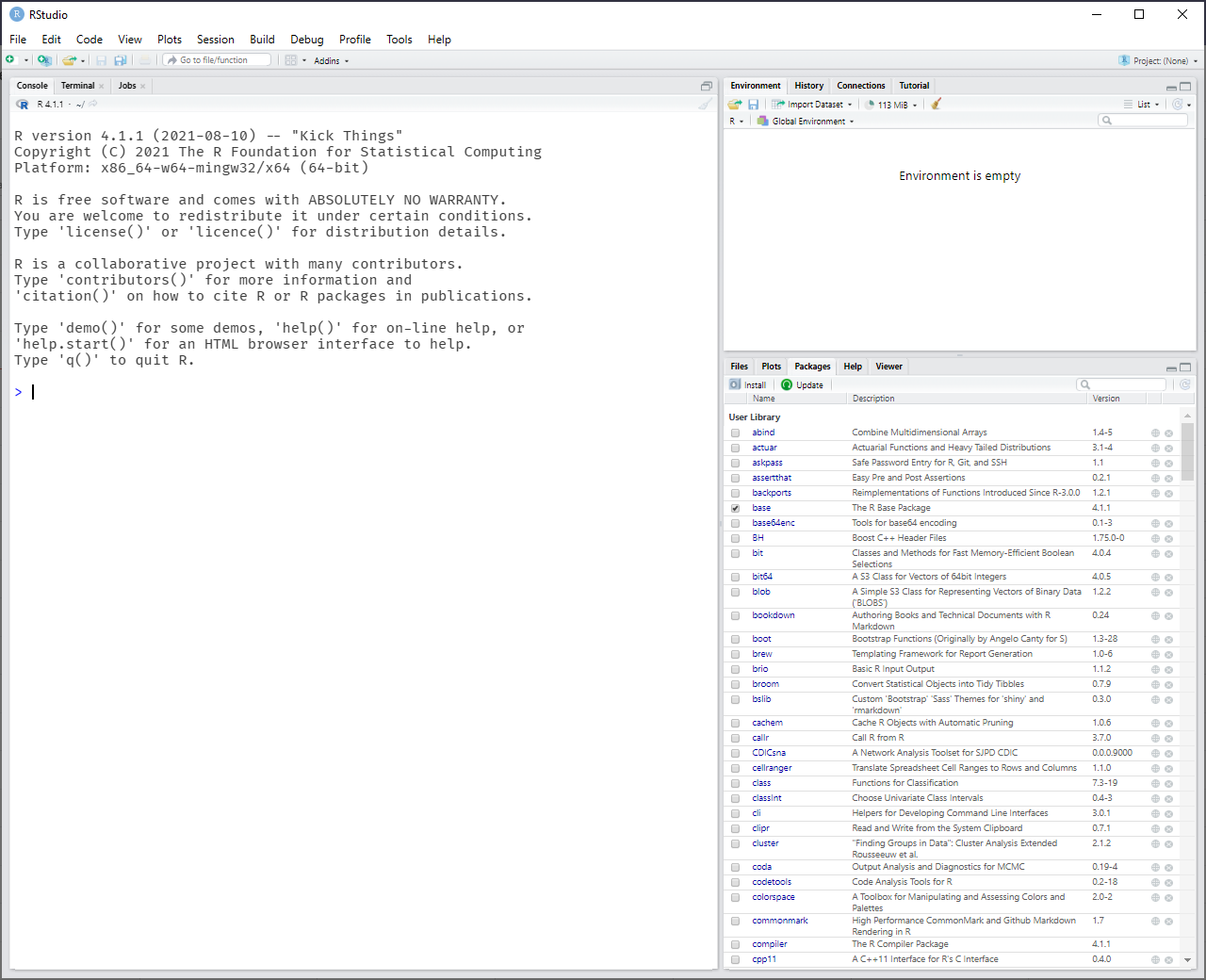
Figure 2.1: Default RStudio Interface
Please note that all panes are movable and can expand or contract. Do not be surprised if they “appear” or “disappear.” Also, the order of panes can be rearranged as some R users prefer changing the position these.
2.1.1 Basics of R Coding in RStudio
Now turn your attention to the Console tab, which is where we interact with the R instance. Any inputs you type into the console will be evaluated and executed in real time. However, you should get in the habit of storing your code for use at a later time. To do so, open an R script, which is plain text file with R commands in it, in order to store your code. Locate the File drop down menu in the top ribbon, navigate to New File, and finally select R Script. Alternatively, press the keys Ctrl + Shift + N (on Mac Cmd + Shift + N). What happened? A new pane should appear with a blank R script, this is where you will write your code prior to executing it.
Now what? Well this document assumes you have some experience working with R. Thus, rather than saturate you with repetitive details on data types and structures, the focus here is on reviewing key functions, best practices, and shortcuts that will improve your efficiency working with R in RStudio. You should consider the following:
- Learning R is much like learning a new language. You may want to start by focusing on a mastering few crucial “words” and “expressions”; then, work your way up to more complex “grammar.” We recommend that familiarize yourself with the following functions as a staring point:
| Function | Description | Example |
|---|---|---|
getwd() |
Return the filepath representing the current working directory of the R process. | getwd() |
setwd() |
Set a working directory for the R process. | setwd("~/PATH") |
install.packages() |
Download and install packages from CRAN-like repositories or from local files. | install.packages(igraph) |
library() |
Load add-on packages. | library(igraph) |
c() |
Combines arguments to form a vector. | c("This", "is", "a", "vector", ".") |
data.frame() |
Creates a data frame. | my_df <- data.frame("Source" = c("Chris"), "Target" = c("Eric")) |
dim() |
Retrieve the dimension of an object. | dim(my_df) |
names() |
Get or set the names of an object. | names(my_df) |
View() |
Invoke a data viewer. | View(my_df) |
class() |
Identify the class an object inherits from. | class(my_df) |
typeof() |
Determine the type of any object. | typeof(my_df) |
head() |
Returns the first part of an object (vector, data frame, etc). | head(my_df) |
NROW() |
Return the number of rows present in a vector, array, or data frame. | NROW(my_df) |
NCOL() |
Return the number of columns present in a vector, array, or data frame. | NCOL(my_df) |
summary() |
Produce result summaries. | summary(my_df) |
read.csv() |
Read file in comma-separated table format and create a data frame from it. | read.csv(~/PATH/MY_FILE.csv) |
write.csv() |
Writes a data frame to a file. | write.csv(my_df, file = "MY_FILE.csv") |
As with any function in R, you may want to look at the documentation for the commands above. This will provide you with additional information the function’s purpose, input arguments, and expected output. To access the documentation for a given function, use the ? operator followed by the function name (e.g., ?help or ?getwd).
All R statements where an object is created are “assignments” and look like this:
object <- value. You can read it, in your head, as “object gets value.” For example,x <- 1is “x gets 1.” You should always use the<-operator in order to avoid confusion. As a suggestion, use spaces surrounding your assignment operator, make it easy to read your code at a later time.Now that you have wrapped your head around assignments, let’s turn to how we name objects. These cannot begin with a digit or contain commas or spaces. Each R user has different a naming convention, we advise you to adopt one of the following:
- Snake Case:
snake_case_object_namefor example:my_object <- 1 - Camel Case:
camelCaseObjectNamefor example:myObject <- 1 - Dots:
dot.object.namefor example:my.object <- 1
Using dots is usually associated with S3 object method dispatching in R (e.g., plot.igraph() plots igraph class objects); thus, many R users avoid using dots to name objects. However, this is not a rule and will not typically impact your code.
- It is highly recommended that you document your code using comments. This practice will allow you to return to your code after time away and just as importantly share your code with others. R allows you to add notes and comments in your scripts and documentation. In order to insert notes or comments into your code, you should use the
#symbol, which tells R to ignore the content to the right of the symbol. For example, notice the difference between the following two commands:
# library(igraph)Vs.
library(igraph) # This will load the igraph library into R's environmentWhat is the difference?
- Code thinking of your future self. The prior two points have hinted this much. Include comments to help explain your thinking and use spacing to improve your code’s readability. For example:
my_df<-data.frame("Source"=c("Chris","Dan","Sean"),"Target"=c("Dan","Sean","Chris")) Vs.
# Create a data frame with two columns (Source and Target) to use as
# an edge list:
my_df <- data.frame(
  "Source" = c("Chris", "Dan", "Sean"),
  "Target" = c("Dan", "Sean", "Chris")
)
Notice the difference? Reading code is hard on a good day, imagine what it would be like to engage with dense and poorly documented code on a bad one.
Remember to leverage the R open-source community! You are probably not the first, nor the last, person learning R. R users are constantly sharing content, collaborating, and asking and answering questions on sites such as StackOverflow or the RStudio Support Site. Google is your friend! Keep in mind that half the battle in solving a problem is finding the right verbiage to describe the issue you have encountered to a search bar. While you should not be afraid to ask questions, you should do your due diligence before starting a new question on either StackOverflow or the RStudio Support Site. Otherwise, you may encounter a less than pleasant user pointing you to the previously asked and answered entry.
Thus far, we have hinted at some keyboard shortcuts built into the RStudio IDE to make the coding experience more pleasant. For example, above we noted the keyboard shortcut to open a new script. There are many more that you may access using Alt + Shift + K, which will bring up a keyboard shortcut reference card. You may want to familiarize yourself with these as they will save you time and improve your experience using RStudio. Here is a list of shortcuts worth knowing:
| Shortcut | Description |
|---|---|
| Ctrl + Shift + N (Cmd + Shift + N on Mac) | Start a new R script. |
| Ctrl + S (Cmd + S on Mac) | Save a script. |
| Ctrl + Shift + C (Cmd + Shift + C on Mac) | Comment or uncomment a line(s) of code. |
| Ctrl + Enter (Cmd + Enter on Mac) | Send a line or multiple lines of code from a script to the console. |
| Ctrl + Alt + R (Cmd + Alt + R on Mac) | Run the complete code in a script. |
2.2 Project Workflow
Up to this point, your analysis has lived in the working directory (see getwd()). This is the location where R looks for files to load and write any outputs. The R user community has moved away from setting working directories ad hoc for a variety of reason; namely:
- Issues with path separators (e.g., \ vs. /) across different operation systems
- Hardcoding paths hinders sharing as no one else will have the same directory as you
To overcome these hurdles, many R users keep all their files for a given project (e.g., class, analysis, etc.) in RStudio Projects. You can create one within RStudio by navigating to the File drop down menu at the top, then selecting New Project. Figure 2.2 shows the step-by-step process of setting up a project. Keep in mind that you can name your project just about anything; however, you should remember two things:
- Name it in a way that reflects the purpose of the project. For instance, if you are setting a project for a class, name it after a class. Names like “my_project” or using your name fail to provide context on the purpose of the project.
- Think carefully about where you put the project, make it easy to find in the future.
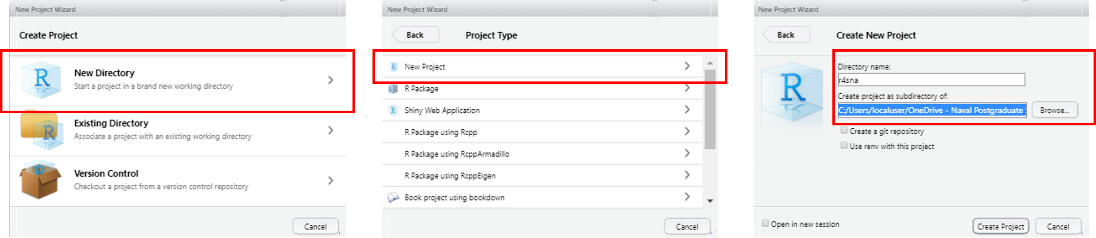
Figure 2.2: Starting an RStudio Project
Once you complete the project setup, check the working directory by executing the following command:
getwd()You should be looking at the path to the project. When you are working in an RStudio Project, your working directory is the location of the project. Thus, as long as you place your data, files, or code inside the project, you won’t have to set and reset the working directory.
For example, let’s create some data and save it. Open a new R script, copy the code below, and execute it:
# First create a data set with random values:
x <- runif(40)
y <- x + rnorm(40, sd = 0.5^2)
my_df <- data.frame("x" = x, "y" = y)
# If you are curious about the distribution of the data, plot it:
plot(my_df$x, my_df$y)
# Now save your data:
write.csv(x = my_df, file = "test_data.csv")
Where did the data write? As noted, it should be located in the project folder your created. If you don’t remember where that may be, use getwd() for a hint. Save the script as “lab0-setup.R” (Ctrl/Cmd + S) and proceed to close your project.
Locate the folder associate with your project, there you should see a file with the extension “.Rproj,” double click on it to reopen RStudio and load your project 2.3.
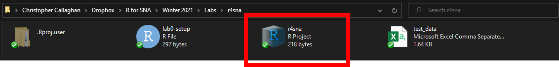
Figure 2.3: Opening RStudio Project
Notice that default, things are restored to where you left them off earlier. Your working directory should still be pointing at the project folder so you could begin your analysis right where you stopped. Furthermore, you won’t have to reset you directory in order to access your data. For example, execute the following command:
read.csv("test_data.csv")Hopefully, you can see the advantage of using RStudio Projects. You may or may not choose to use them in this class. However, you should be aware of them and their added advantages as they are commonly used by R users to power their analysis.