7 Network Topography in igraph
7.1 Setup
Find and open your RStudio Project associated with this class. Begin by opening a new script. It’s generally a good idea to place a header at the top of your scripts that tell you what the script does, its name, etc.
#################################################
# What: Network Topography in R
# Created: 02.28.14
# Revised: 01.18.22
#################################################
If you have not set up your RStudio Project to clear the workspace on exit, your environment contain the objects and functions from your prior session. To clear these before beginning use the following command.
rm(list = ls())Proceed to place the data required for this lab (Anabaptists Leaders.csv, and Anabaptists Attributes.csv) also inside your R Project folder. We have placed it in a sub folder titled data for organizational purposes; however, this is not necessary.
For this exercise, we’ll use the Anabaptist Leadership network and its related attribute data, both of which can be found in the file we shared with you. The data set includes 67 actors, 55 who were sixteenth century Anabaptist leaders and 12 who were prominent Protestant Reformation leaders who had contact with and influenced some of the Anabaptist leaders included in this data set. These network data build upon a smaller dataset (Matthews et al. 2013) that did not include some leading Anabaptist leaders, such as Menno Simons, who is generally seen as the “founder” of the Amish and Mennonites.
We will add a measure here not implemented in the statnet version of this lab, namely the clustering coefficient. A few versions exist but it is conceptually similar to other measures of interconnectedness.
7.2 Load Libraries
Load igraph library.
library(igraph)It is not currently possible to calculate the E-I index in statnet and igraph, but a package, isnar, has been developed to do just that. Its functionality is demonstrated at the end of this lab. We’ve included the scripts in both statnet and igraph versions of this lab, but you need to do this section only once.
In addition to igraph, we will be introducing and using isnar. Since this may be the first time you are using this tool, please ensure you install it prior to loading it. You will need to install remotes in order to use the function install_github() to download and set up isnar as it is not published on the CRAN.
install.packages("remotes")Now install isnar.
remotes::install_github("mbojan/isnar")Before moving forward, let’s load the isnar package:
library(isnar)Note: igraph imports the %>% operator on load (library(igraph)). This series of exercises leverages the operator because we find it very useful in chaining functions. We occasionally show how to carry out a series of commands with and without piping.
7.3 Import Data
Let’s import the data using the read.csv() function. Remember, igraph’s graph_adjacency() function requires a matrix.
anabaptist_matrix <- read.csv("data/Anabaptist Leaders.csv",
                              header = TRUE,
                              row.names = 1,
                              check.names = FALSE) %>%
  as.matrix()
Now transform the matrix to an igraph object.
anabaptist_ig <- graph.adjacency(anabaptist_matrix,
                                 mode = "undirected")

anabaptist_ig
IGRAPH b43b453 UN-- 67 183 --
+ attr: name (v/c)
+ edges from b43b453 (vertex names):
[1] Martin Luther --Ulrich Zwingli Martin Luther --Thomas Muntzer
[3] Martin Luther --Andreas Carlstadt Martin Luther --Caspar Schwenckfeld
[5] Martin Luther --Melchior Hofmann Martin Luther --Philipp Melanchthon
[7] Martin Luther --Martin Bucer John Calvin --Wolfgang Capito
[9] John Calvin --Martin Bucer Ulrich Zwingli--Joachim Vadian
[11] Ulrich Zwingli--Conrad Grebel Ulrich Zwingli--Felix Manz
[13] Ulrich Zwingli--George Blaurock Ulrich Zwingli--Wilhelm Reublin
[15] Ulrich Zwingli--Johannes Brotli Ulrich Zwingli--Louis Haetzer
+ ... omitted several edgesTo correctly calculate a number of topographical metrics in igraph (e.g., centralization), we need to make sure that the network is a “simple” graph/network, that is, a network without multiple lines or loops (diagonal). We can check whether the Anabaptist network is a simple graph with the following command:
is_simple(anabaptist_ig)[1] TRUEWe can see that it is already a simple graph, so we don’t have to simplify it. However, if we need to, we would issue the following command:
simplify(anabaptist_ig,
         remove.multiple = TRUE,
         remove.loops = TRUE,
         )
IGRAPH b44928c UN-- 67 183 --
+ attr: name (v/c)
+ edges from b44928c (vertex names):
[1] Martin Luther --Ulrich Zwingli Martin Luther --Thomas Muntzer
[3] Martin Luther --Andreas Carlstadt Martin Luther --Caspar Schwenckfeld
[5] Martin Luther --Melchior Hofmann Martin Luther --Philipp Melanchthon
[7] Martin Luther --Martin Bucer John Calvin --Wolfgang Capito
[9] John Calvin --Martin Bucer Ulrich Zwingli--Joachim Vadian
[11] Ulrich Zwingli--Conrad Grebel Ulrich Zwingli--Felix Manz
[13] Ulrich Zwingli--George Blaurock Ulrich Zwingli--Wilhelm Reublin
[15] Ulrich Zwingli--Johannes Brotli Ulrich Zwingli--Louis Haetzer
+ ... omitted several edgesNote that the defaults for the remove.multiple and remove.loops options are TRUE, so we didn’t really need to include them in the previous command.
7.4 Network Size and Interconnectedness
7.4.1 Network Size
Network size is a basic descriptive statistic that is important to know because many of the subsequent measures are sensitive to it. Network size is easy to get with the vcount() function. As you may have noticed, you get the network size as well when you call the igraph object anabaptist_ig, which is what we just did in the previous step.
vcount(anabaptist_ig)[1] 677.4.2 Density and Average Degree
Network density equals actual ties divided by all possible ties. However, density tends to decrease as social networks get larger because the number of possible ties increases exponentially, whereas the number of ties that each actor can maintain tends to be limited. Consequently, we can only use it to compare networks of the same size. An alternative to network density is average degree centrality, which is not sensitive to network size and thus can be used to compare different sized networks.
First, calculate density using density using the edge_density() function.
edge_density(anabaptist_ig)[1] 0.08276798In order to calculate the average degree centrality, you will have to calculate vertex degree and proceed taking the average of this vector of scores.
degree(anabaptist_ig) %>%
  mean()
[1] 5.462687You can also do this not using pipes:
mean(degree(anabaptist_ig))[1] 5.462687Keep in mind that you may continue refining the output by rounding the value:
edge_density(anabaptist_ig) %>%
  round(digits = 3)
[1] 0.083degree(anabaptist_ig) %>%
mean() %>%
round(digits = 3)[1] 5.4637.4.3 Clustering Coefficient (Global and Local)
To calculate this measure, use the transitivity() function. This measure can be calculated for each vertex (type = "local") or as a ratio of triangles and the connected triples in the graph (type = "global").
# Traditional transitive measure:
transitivity(anabaptist_ig,
             type = "global")
[1] 0.3557214# Local transitive scores (for each ego):
transitivity(anabaptist_ig,
type = "local") [1] 0.2857143 1.0000000 0.1923077 0.3333333 0.3818182 0.6666667 0.2380952
[8] 0.2527473 0.6666667 0.4000000 1.0000000 1.0000000 1.0000000 1.0000000
[15] 0.2222222 0.3333333 0.5000000 0.2545455 0.2166667 0.5000000 0.2142857
[22] 0.7000000 0.3888889 0.3333333 0.2500000 0.3333333 1.0000000 0.3214286
[29] 0.4285714 0.4285714 0.3928571 0.5000000 0.7619048 0.8000000 0.8666667
[36] 0.3571429 NaN 0.0000000 0.0000000 NaN 0.8333333 0.5000000
[43] NaN 0.4000000 1.0000000 0.0000000 0.1666667 0.4444444 0.4444444
[50] 1.0000000 NaN 0.4722222 0.4444444 0.5000000 0.2380952 0.5000000
[57] 1.0000000 0.3333333 0.5000000 0.0000000 0.3000000 0.0000000 0.3333333
[64] 0.3111111 0.3111111 NaN 0.0000000Notice the NaN values (not a number). We can take the average of local clustering coefficients and ignore these missing values by combining this function with the mean() function.
mean(
  transitivity(anabaptist_ig,
               type = "local"),
  na.rm = TRUE
)
[1] 0.4605426Alternatively, rather than removing the NaN we could zero them out and include them in the calculation of an average clustering coefficient. This is how ORA calculates the measure.
trans <- transitivity(anabaptist_ig,
                      type = "local")
# Calculate the mean:
mean(
  # Recode trans vector, if NaN assing 0, otherwise return value
  sapply(trans, function(s) ifelse(is.nan(s), 0, s))
  )
[1] 0.42617377.4.4 Cohesion and Fragmentation
Now we turn to some additional measures related to the concept of interconnectedness.
cohesion(anabaptist_ig)[1] 1Because the network is not disconnected, cohesion is 1.00 and fragmentation is 0.00. However, with a little manipulation, we can also compute distance weighted cohesion and fragmentation, what is often called compactness and breadth.
First, calculate length of all shortest paths from or to the vertices in the graph.
anabaptist_dist <- distance_table(anabaptist_ig,
                                  directed = FALSE)
The distance_table() function returns a named list with two objects. The first, res, is a numeric vector of distances. The second, unconnected, the number of unconnected pairs. The sum of the two is always n(n-1) for directed graphs and n(n-1)/2 for undirected graphs, which is the number of potential pairs in a network.
Cohesion can be calculated by adding the number of connected pairs divided by the total number of possible pairs in the network.
# Calculate cohesion
sum(anabaptist_dist$res) /
  (sum(anabaptist_dist$res) + anabaptist_dist$unconnected)
[1] 1Calculating the fragmentation is as simple as removing the cohesion score from 1.
# Calculate fragmentation
1 - sum(anabaptist_dist$res) /
  (sum(anabaptist_dist$res) + anabaptist_dist$unconnected)
[1] 07.4.5 Compactness and Breadth
igraph has no direct way to calculate compactness. However, here is how to compute compactness and breadth using the available tools from igraph.
First, calculate the length of all the shortest paths for all vertices in the network.
distance <- distances(anabaptist_ig)Take a look at the matrix of distances, here only the first four rows and columns:
distance[1:4, 1:4] Martin Luther John Calvin Ulrich Zwingli Joachim Vadian
Martin Luther 0 2 1 2
John Calvin 2 0 2 3
Ulrich Zwingli 1 2 0 1
Joachim Vadian 2 3 1 0We can read these distances as steps between nodes. So Martin Luther is two steps away from John Calvin.
Calculating compactness requires calculating the reciprocal distance by taking the inverse of the distances in the matrix, removing the diagonal containing self distance scores and replacing infinite distances (disconnected nodes listed as Inf) with a zero. Then taking the mean of all reciprocal distances in the matrix.
# Calculate reciprocal distances
reciprocal_distances <- 1/distance
# Modify the reciprocal_distances matrix
diag(reciprocal_distances) <- NA
reciprocal_distances[reciprocal_distances == Inf] <- 0
# Calculate compactness
compactness <- mean(reciprocal_distances, na.rm = TRUE)
compactness
[1] 0.3800372For breadth, we could, of course, just take the additive inverse of compactness.
breadth <- 1 - compactness
breadth
[1] 0.61996287.5 Centralization and Related Measures of Spread
Network centralization, variance, and standard deviation are measures that can capture the hierarchical dimension of a network’s topography. Centralization uses the variation in actor centrality (as compared to the highest centrality score) within the network to measure the level of centralization. More variation yields higher network centralization scores, while less yields lower scores. In general, the larger a centralization index is, the more likely it is that a single actor is very central while the other actors are not. Thus, the index can be seen as measuring how unequal the distribution of individual actor scores are. Because we can calculate centralization using different measures of centrality (e.g., degree, betweenness, closeness, and eigenvector), we need to interpret the results in light of the type of centrality used. Centralization scores range from 0.00 – 1.00 (or 0 – 100%) when analyzing dichotomized data. If you are analyzing valued data, centralization scores will sometimes be larger than 1.00; thus, it’s generally a good idea to dichotomize your data before estimating network centralization.
7.5.1 Centralization
Here’s how to get centralization scores for the four primary measures of centrality that we’ve discussed in previous classes.
Let’s begin taking a look at how to calculate degree centralization, which is accomplished in igraph through the centralization.degree() function. It takes an igraph object as input and return a named list with three components:
res: a numeric vector containing the node-level degree centrality score for all vertices in a graphcentralization: a graph level centrality indextheoretical_max: The theoretical maximum graph level centralization for a graph with the given number of nodes
Since we are looking for topographical or network level measures, the focus here is on extracting the centralization component from the output.
# First calculate the centralization
anabaptist_deg_cent <- centralization.degree(anabaptist_ig, loops = FALSE)
# Now return the named component of interest
anabaptist_deg_cent$centralization
[1] 0.1645688You could assign the centralization score to an object, or bypass this step and just call it by attaching a $ accessor and the named component to the function call.
# Calculate betweenness centralization
centralization.betweenness(anabaptist_ig)$centralization
[1] 0.1974781Here is the last two remaining centralization functions.
# Calculate closensess centralization
centralization.closeness(anabaptist_ig)$centralization
[1] 0.2199767# Calculate eigenvector centralization
centralization.evcent(anabaptist_ig, scale = FALSE)$centralization[1] 0.30677727.5.2 Variance and Standard Deviation
Variance and standard deviation are similar to centralization. They differ from centralization in that rather comparing individual scores to the highest centrality score, they compare individual scores to the average centrality score. Because standard deviation is the square root of the variance, it is probably preferable to variance because it returns to the original unit of measure.
Here’s how to get the standard deviation of the network. To do so, you will have to provide the sd() function with a numeric vector, which will represent the node level measures (e.g., degree centrality (degree()), closeness (closeness()), etc.).
Let’s begin by setting up the code to calculate the standard deviation for the anabaptist_ig graph based on degree centrality.
# Calculate standard deviation
sd(
  # Provide the numeric vector of degree scores
  degree(anabaptist_ig,
         # Ignore loop edges
         loops = FALSE)
  )
[1] 3.434797Now calculate the standard deviation for closeness, betweenness, and eigenvector centrality.
sd(
  closeness(anabaptist_ig,
            normalized = TRUE)
  )
[1] 0.05769685sd(
betweenness(anabaptist_ig)
)[1] 110.4204sd(
# Returns a named list, with the centrality scores in the vector component
evcent(anabaptist_ig,
scale = FALSE)$vector
)[1] 0.0801868A drawback of standard deviation…
sd.deg <- sd(degree(anabaptist_ig))
sd.clo <- sd(closeness(anabaptist_ig, normalized = TRUE))
sd.bet <- sd(betweenness(anabaptist_ig))
sd.eig <- sd(evcent(anabaptist_ig, scale = TRUE)$vector)

# Create a star graph with the same number of actors
star.ig <- make_star(vcount(anabaptist_ig), mode = "undirected")
plot(star.ig)

# Standard deviation of star graphs
starsd.deg <- sd(degree(star.ig))
starsd.clo <- sd(closeness(star.ig, normalized = TRUE))
starsd.bet <- sd(betweenness(star.ig))
starsd.eig <- sd(evcent(star.ig, scale = TRUE)$vector)

# Divide the first by the second
sd.deg/starsd.deg
[1] 0.4325388sd.clo/starsd.clo[1] 0.9518038sd.bet/starsd.bet[1] 0.421366sd.eig/starsd.eig[1] 2.469133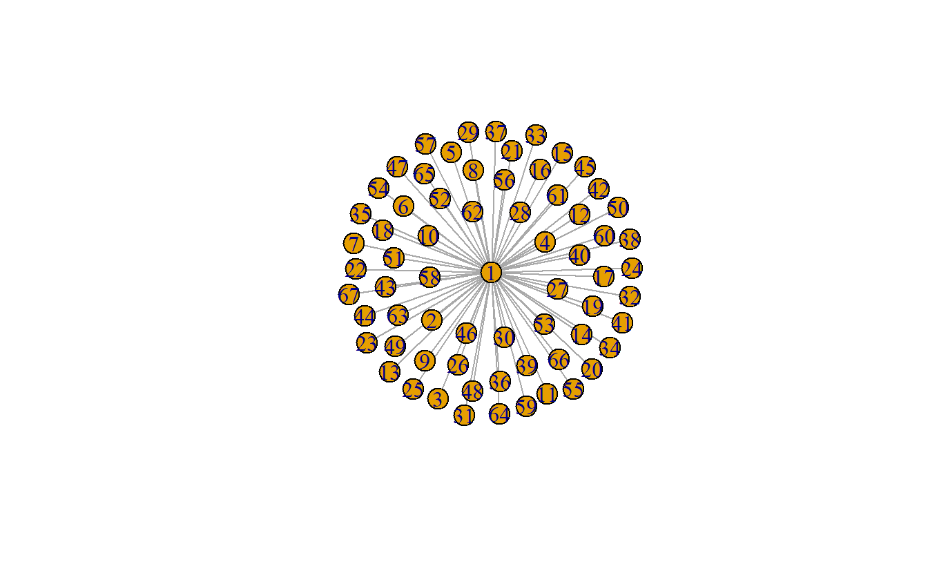
7.5.3 Diameter and Average Path Distance
Here’s how to get geodesic information on a network and then use it to calculate average distance and diameter.
The diameter is the longest of all shortest paths that traverse the network. It is calculated in igraph using the diameter() function.
diameter(anabaptist_ig,
         directed = FALSE,
         unconnected = FALSE)
[1] 9The average path length is the shortest paths between all actors in the network. It is calculated in igraph using the average.path.lenght() function.
average.path.length(anabaptist_ig)[1] 3.3541387.6 Calculating the E-I Index with isnar
This section is in both statnet and igraph versions of this lab. You only need to do this section one time.
E-I Index indicate the ration of ties a group has to nongroup members. The index equals 1.0 for groups that have all external ties, while a group with -1.0 score has all internal ties. If the internal and external ties are equal, the index equals 0.0.
The E-I Index is not common to many R packages, and it is not as simple as one would think it would be to program. However, there is a package called isnar that does calculate it (Bojanowski 2021). It is written and maintained by Michal Bojanowski (m.bojanowski@icm.edu.pl) as a supplement to igraph. The only thing is that isnar is only available through GitHub. GitHub is a repository for open-source software, like R packages in development.
To estimate the E-I index, we require an attribute vector. Here, we’ll use the Melchiorite attribute included in the attribute file.
attributes <- read.csv("data/Anabaptist Attributes.csv",
                       header = TRUE)
Take a look at the vector names.
names(attributes) [1] "ï..Names" "Believers.Baptism" "Violence"
[4] "Munster.Rebellion" "Apocalyptic" "Anabaptist"
[7] "Melchiorite" "Swiss.Brethren" "Denck"
[10] "Hut" "Hutterite" "Other.Anabaptist"
[13] "Lutheran" "Reformed" "Other.Protestant"
[16] "Tradition" "Origin.." "Operate.." The Melchiorite vector can be accessed using the [[ accessor. Now, use the ei() function to get the E-I index.
ei(anabaptist_ig, attributes[["Melchiorite"]],
   loops = FALSE, directed = FALSE)
[1] -0.93442627.7 Network Level Measures Table
You may want to export out these measures as a table for your report. Luckily, we can use a data.frame to capture the data in a tabular format, then export it out as a CSV.
# First, create a data.frame of outputs
net_topography <- data.frame(
  `size` = vcount(anabaptist_ig),
  `average distance` = average.path.length(anabaptist_ig),
  `diameter` = diameter(anabaptist_ig),
  `degree centralization` = centralization.degree(anabaptist_ig)$centralization,
  `standard deviation` = sd(degree(anabaptist_ig)),
  `density` = edge_density(anabaptist_ig),
  `average degree` = mean(degree(anabaptist_ig)),
  `global clustering coefficient` = transitivity(anabaptist_ig, type = "global")
)
Take a look at the output:
str(net_topography)'data.frame': 1 obs. of 8 variables:
$ size : int 67
$ average.distance : num 3.35
$ diameter : num 9
$ degree.centralization : num 0.16
$ standard.deviation : num 3.43
$ density : num 0.0828
$ average.degree : num 5.46
$ global.clustering.coefficient: num 0.356Export it out.
write.csv(net_topography, file = "network_topography.csv", row.names = FALSE)That’s all for igraph now.